Date Spread

Recently I had a couple of interesting situations pop up in OBIEE 11g regarding dates. No not the edible kind, but the calendar kind. Specifically where it involves fact measures that are valid for a period of time beyond what the date id(s) on the rows in the table allow. The first scenario I will go through is when you want the measure applied over an entire year, but there is only one record. For example, a date_id of 20160101 that represents the entire year of 2016. The second scenario involves having two dates (like a start date and an end date) but for analysis I want to be able to pick any date in between those dates and have it still bring back results.

The solution for these situations is to “spread” the dates via a complex join from the fact to the date dimension. These will get spread in different ways, but the end result is the same. Beware that if your analysis is at a grain higher than the date level, you will have multiplicity issues. The solution to this is to do aggregation based on dimensions; don’t worry… I’ll also an example of this later in the post.

Scenario 1

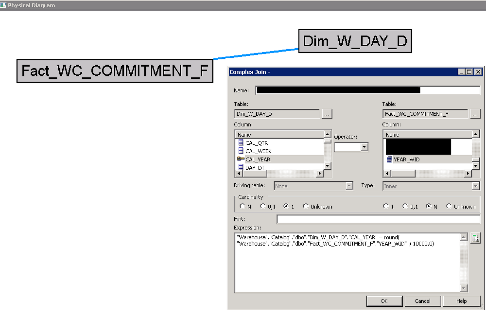
I had a situation where a dealer would commit to selling a certain number of units in the calendar year. This would get input into the database as a single record with a YEAR_WID format of YYYYMMDD. When I created an analysis, this would then only show up as a single point on a chart for the whole year. This wouldn’t get us very far if we think in terms of a larger, conformed model. What I really want is to express this as a line across the visualization for an entire year. So without making any changes to the data model, I created my own year field in the join. By dividing the YEAR_WID by 10,000 and then rounding the remaining decimal off, I was left with just the YYYY portion of the original WID, which could then be joined to W_DAY_D.CAL_YEAR.

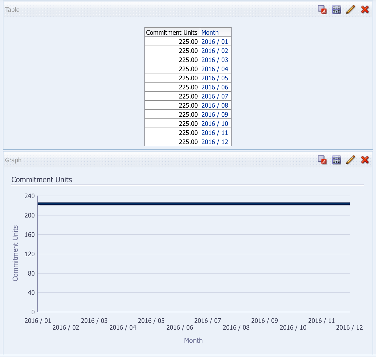
Now instead of a single point in time, I get the same result for all days of the year, which gives me the straight line I wanted in my chart. More importantly, if I am combining this with facts from another table, I can use any date and will still be able to bring the Commitment Units into that analysis.

Scenario 2

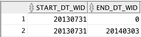
The second situation I had was with a different fact table used for inventory reorder. The product dealer has an auto reorder level that is set for a specified period of time. Each row has a start date and an end date. If the END_DT_WID = 0 then the inventory reorder record is still active; if there is a date then it is no longer active and was only active between the start date and end date.

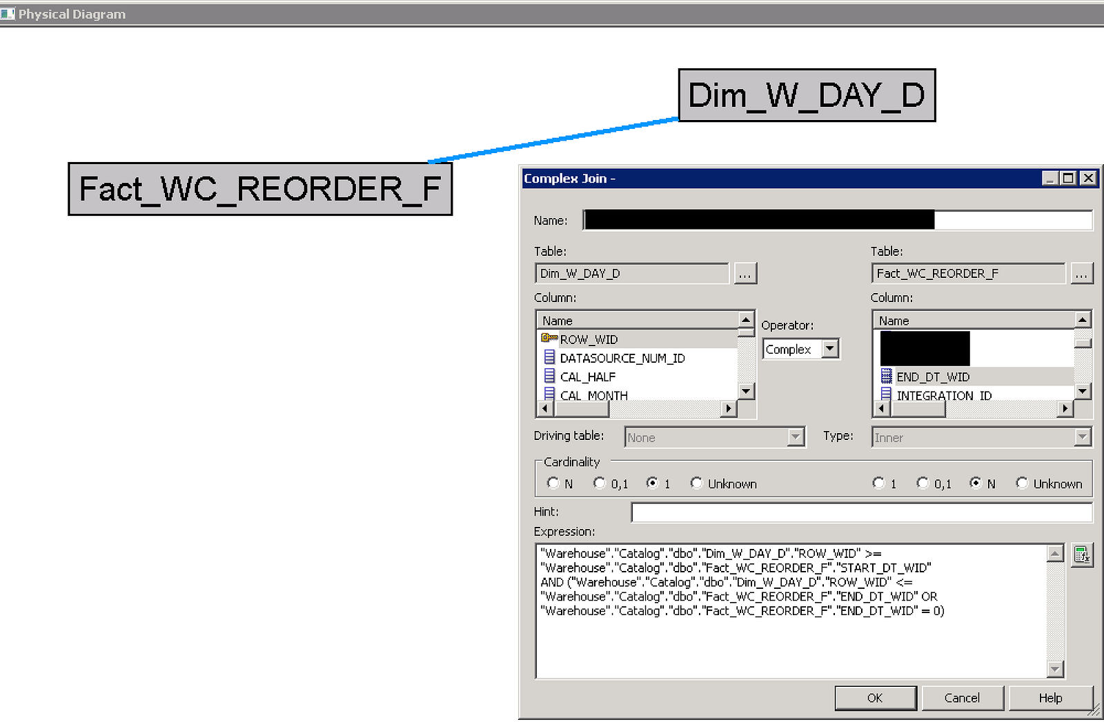
Similar to the first situation, I wanted to see this reorder point across any date that is between the start date and end date; with the original setup, this wasn’t possible. Again I didn’t want to try to reengineer the data model to make this work that way, so I used another complex join from the fact to the date table with the following logic.

(W_DAY_D.ROW_WID >= WC_REORDER_F.START_DT_WID
AND
W_DAY_D.ROW_WID <= WC_REORDER_F.END_DT_WID)
OR
WC_REORDER_F.END_DT_WID = 0

By doing this join I can now use my date dimension with this fact the way I would other fact tables. For example, if I picked 01/01/2014 I would see results for all records that were active at that point in time, whether or not they are still active.

The thing to remember is that when doing complex joins like these examples, you are artificially creating records for every day within your analysis criteria. What this means is that you will only get back the correct results when at the day level. However, this can be solved by doing aggregation based on dimensions. This allows you to set different aggregation rules for different dimensions.

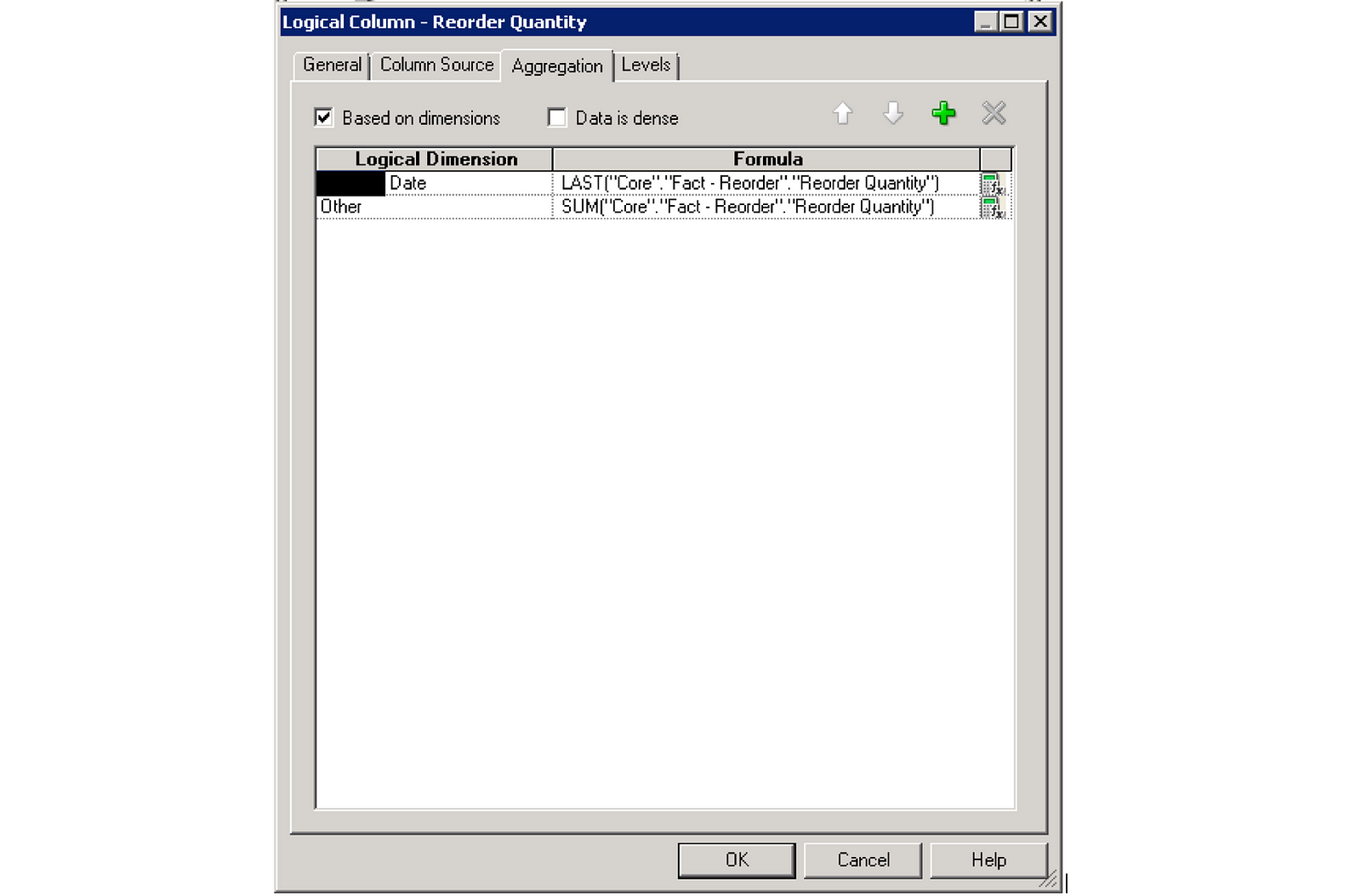
For each metric from the logical fact table where multiplicity will be an issue, you will need to set this rule. In the case of reorder quantity, the multiplicy issue only comes into play on the Date dimension. Because of this, I want to apply LAST() to the date dimension so that it just picks the last record for the given level of detail. For Example, if my report is at the month level, it will just pick the last day of the month. I still want it to sum by every other dimension, so I can simply just leave it at SUM() for Other.

The important thing to remember with aggregation based on dimensions is that for every dimension you explicitly apply an aggregation rule to (any dimension listed that isn’t Other), this will get pulled into your query SQL, regardless of whether it is in your analysis which can negatively impact performance. Thus, it is best used when you only have one or 2 dimensions that need special aggregation rules applied.

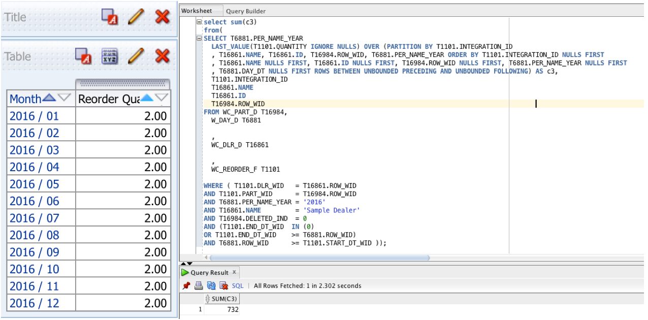
The analysis on the left shows the aggregation based on dimensions working, so no matter if I am at day, month, quarter, or year, I will always get 2 (the right answer). If I only had SUM(Reorder Quantity), which I demonstrated by summing the query for all of 2016, it returns 732, which is 2*366 days since 2016 is a leap year.

Spreading dates like this is not something you will likely see very often, but can come in handy from time to time. Hopefully, if you have an issue similar to this, you can follow the steps in this post to get the numbers you want.