
As I’ve been discussing in my last few blogs, it’s possible to start using OBIEE for analytics, rather than the standard operational reporting and BI that is commonplace. Data science has been quite the buzz the last few years, and no doubt about it, data scientists can bring great value and understanding to an organization, serve as ambassadors for analytics and contribute to a data driven culture. According to Forbes, data scientists spend most of their time preparing data, rather than analyzing it. Sometimes, this preparation involves identifying outliers within a data set. Within the suite of 12c’s analytical tools is the Outlier function, which will help analysts and scientists alike identify and remove the noise within the data.
What is an Outlier?
An outlier is a data point that is outside the normal distribution of data as a whole. What this means in layperson’s terms is that the outlier point is distant from the collection of other data points. Sometimes outliers are due to error (either in an experiment or in measurement), but it is also entirely possible that outliers are valid data points that do not fit the standard mold, or curve, of the data. Because of this, use care when omitting outliers from your data sets; just because they are not part of a normal distribution does not mean that they do not have meaning! You may want to omit outliers if you are trying to find the mean for a data set — this can remove skew in one direction or another and better represent what is “normal”. However, you may want to keep outliers in a data set if you are trying to understand patterns or behavior; sometimes these outliers highlight something different that is worth noting and learning from.
OBIEE’s Outlier function works similarly to the cluster function that I discussed in an earlier blog post, however there are some distinct differences in how these functions work and their outputs. Where the Cluster function will assign a cluster name or number to each grouping, the Outlier function will assign either TRUE or FALSE to each value, based on the value’s normality. This is accomplished via several clustering algorithms that can be specified in the function’s parameters; those algorithms are described in detail below.
K-Means clustering attempts to create a cluster by finding the mean distance between all data points. It then finds the center of a cluster with the shortest distance between each centroid (the center) and each data point: points that are assigned to whichever cluster they are closest to. Once these assignments have been made, the algorithm can iterate based on an iteration counter. By doing this iteration and re-running the algorithm, the clusters’ centroids are repositioned and distances between the data points are remeasured. Based on the new outputs, this potentially associates new data points that are closer to to the new centroid. Points that are further away from other centriods are added to the outlier grouping.
Hierarchical clustering does exactly what the name suggests — it creates clusters based on hierarchy. The data is clustered from either a top-down or bottom-up approach, and is determined by distance between data points, as with K-Means. Unlike K-Means however, these distances are measured from the direction in which the algorithm is being executed. Data points further away are identified as outliers, as in K-Means.
Multivariate Outlier Detection is the default algorithm for the Outlier function, and is based on the Mahalanobis distance of each data point. The Mahalanobis distance is the number of standard deviations between the data point and the normal distribution. This measurement technique is especially helpful in multidimensional situations because no matter the number of axes in play, it will always measure along the normal distribution and calculate the deviation of that distribution — thus identifying the outliers.
The Outlier Function
Now that we have the concepts down, let’s take a look at how to use the function. The function’s syntax is below, followed by the breakdown of the parameters.
OUTLIER( (dimension_expr1 , ... dimension_exprN), (expr1, .. exprN),
output_column_name, options, [runtime_binded_options] )
The first parameter, dimension_expr, is the input parameter for the dimensions you wish to use in your outlier detection. This is a list of dimensional columns.
The expr parameter is a list of fact columns that you wish to perform the outlier detection on.
The output_column_name parameter alters the function’s output value. Select ‘isOutlier’ for the ‘TRUE’ or ‘FALSE’ value for the data point, or use the ‘distance’ value to see the distance (the units and calculation of which will change depending on the algorithm you use).
options allow for more fine tuning of the Outlier function, with several additional parameters available for use. These parameters and their values should be enclosed in single quotes and separated with semi-colons. The optional parameters are outlined below.
‘attributeName’ is a list of other attributes to use in outlier detection. These inputs are separated by commas.
‘algorithm’ is the name of the algorithm you wish to use for your outlier detection (remember, I discussed the differences in algorithms above). The available values are ‘mvoutlier’, ‘h-clustering’ and ‘k-means’. Keep in mind that ‘mvoutlier’ is the default, and will be specified if you do not change the algorithm with this parameter.
The ‘useRandomSeed’ is the option that determines the starting point for the initial iteration. If set to ‘TRUE’, then each time the analysis is run, it will generate a random starting point; if it is set to ‘FALSE’, the value will be stored and the results will be reproducible. ‘TRUE’ is recommended for production environments, and ‘FALSE’ is recommended for DEV or QA for testing purposes.
‘initialSeed’ is used when the ‘useRandomSeed’ value is set to ‘FALSE’. This value is an integer, with a default of 250 if omitted.
The ‘isTopNAsPercentage’ parameter controls how the outlier points are determined, and could be seen as a function override. If set to ‘FALSE’, then the algorithm is allowed to run without interference. This is the default behavior. If set to ‘TRUE’, then the outliers will be determined by taking the top N percent of the algorithm’s output. The value of the percentage is determined in the ‘topN’ optional parameter (see below). (A digression on this option: I tried to use this parameter and was returned the following error: [nQSError: 23072] Missing alias/option isTopNAsPercentage in the script file filerepo://obiee.Outliers.xml (HY000). It is included in the Oracle documentation, but I have a feeling that the option is named differently than seen there. I will update this blog if I discover what it is.)
‘topN’ is only used when the ‘isTopNAsPercentage’ is set to ‘TRUE’. The input value is a double data type, and the default is 3 if the parameter is omitted.
The runtime_binded_options is an optional parameter for the Outlier function, and allows the seeding of values into the function’s parameters at run time. These are comma separated values that correspond to the defined options in the function. To enable, each option you would like to run at run time must equal %N, where N is the position in the list of runtime options.
Let’s take a look at an Outlier example; both the syntax and the output. (For those of you following along at home, I am using Oracle’s Sample App v607).
OUTLIER( ("Products"."P4 Brand", "Products"."P1 Product"), ("Base Facts"."1- Revenue", "Base Facts"."3- Discount Amount"), 'isOutlier', 'algorithm=%1;useRandomSeed=%2;', 'mvoutlier', 'FALSE')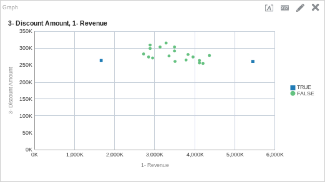
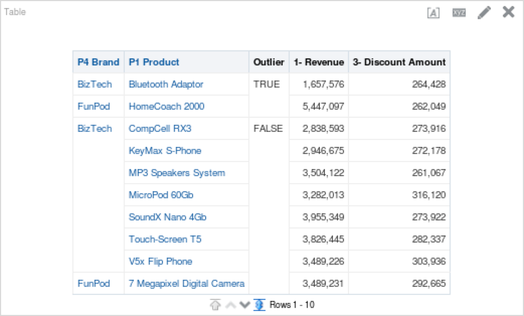
You’ll notice above that the outlier function did an excellent job of pointing out which data would be considered an outlier, and which is part of the normal set. Remember, just because a data point is an outlier does not mean that is it meaningless. Below is a table that shows outlier points above. My take away from the table is that Bluetooth Adaptors require more discounting and the HomeCoach 2000 does not. We can also see that HomeCoach 200o is a revenue leader, while Bluetooth Adaptors are far below other products in terms of revenue generation.
Now that we’ve got a handle on how the Outlier function works, let’s work through a few more examples, shall we?
Play It Again
This time, let’s depart from the standard revenue and discount example, and think outside the box. Let’s investigate whether or not we have any outliers between our target and billed quantities for each product and office. As 2015 is the most recent year in the data set, let’s begin by filtering on that, and see what we can learn. Below is the outlier function I used.
OUTLIER( ("Products"."P1 Product", "Offices"."D1 Office"), ("Base Facts"."2- Billed Quantity", "Base Facts"."6- Target Quantity"), 'isOutlier', 'algorithm=%1;useRandomSeed=%2', 'mvoutlier', 'FALSE')Let’s put this on a scatter plot and see what is looks like.

Now the fun begins; let’s try to make some sense of what is happening above. Unlike the first example, this is a little more intensive. It is important to keep in mind that the outlier function will find outliers based on distance from the distribution curve. This is especially important to remember when we see plots like the one above, where things can seem initially confusing with outliers so close to non-outlier points. The first thing to note is that this curve would be skewed right, as there are more outlier points along the right side of the plot.
Another observation we can make quickly is that almost universally, the target quantities are magnitudes higher than the billed quantities. Some of these more extreme cases are highlighted as outliers above. We can also note that there is a block of points that have higher success ratios than the rest (see graph below).

To make some more sense of it all, let’s put it into a table, which is below. I also created a new metric to measure the percentage of billed quantity to target quantity. I sorted descending on “Outlier?” and the “Billed to Target Percentage” columns.
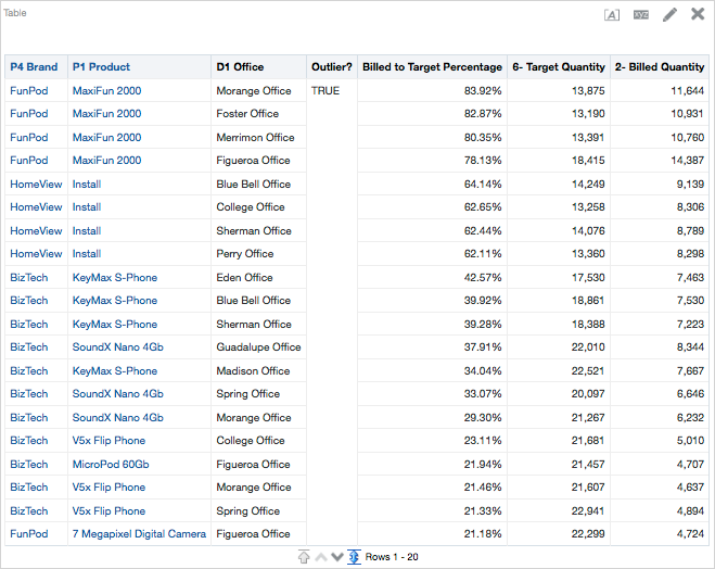
Now that we have our data in a table, we can more easily quantify differences. We could sort the data N ways to Sunday to see potential relationships. Which offices have higher success rates? Which products have more outliers? Why do they have more outliers? We could also add richness to the analysis by bringing in sales person columns, customer columns, or order information. The main point here is to start asking questions and trying to find answers. Sometimes, these answers can be easy to discern, but other times, they can be more difficult.
At this point I would try to engage with the business and get a sense for why things turned out the way they did in 2015. I would ask questions like “Why were some targets so high?”, “Was there a shift in business strategy part way through the year?”, “Were some products discontinued in specific locales?”. These types of questions can lend answers that are not readily available from the data. Along with the Forecast function, the Outlier function could provide great insight into potential business opportunities and challenges.
Like many of the other functions in OBIEE 12c’s analytics suite, the Outlier function is a starting point. It allows users to identify points that are outside the norm, and ask questions about the data.