Cluster Func 

Clustering. Whether we’re talking about headaches, compute nodes, or uh, well, I’ll let you fill in the blank… isn’t anything worth doing, worth doing together? Clustering can be a powerful tool for understanding the relationships between data, and in this post I’ll walk through how to use the OBIEE 12c Advanced Analytics Cluster Function. As a reminder, you will need to have the R packages installed and enabled on your OBIEE 12c instance to use this function! (I’ll have a blog post on this in the near future.)

C.L.U.S.T.E.R.

Before I jump into the function’s syntax and properties, let’s first discuss what a cluster is, and why it is important. The purpose of any clustering analysis is to determine simplified and similar groups based on observations (facts or measures) along dimensional attributes. Each group — a cluster — should maximize the similarities within it, while minimizing the similarities between other clusters. While this seems simple on the surface, sometimes creating these types of groupings can be difficult when attemping to sift through thousands or even millions of rows manually. A good example of this would be to determine groups of customers based on their buying patterns. How does this actually work though?

There are many different ways to calculate clusters from a statistical standpoint, but for the sake of simplicity OBIEE’s Cluster function only supports two methodologies at the moment: K-Means and Hierarchical.

K-Means clustering attempts to create a cluster by finding the mean distance between all data points. It then finds the center of a cluster with the shortest distance between each centroid (the center) and each data point: points that are assigned to whichever cluster they are closest to. Once these assignments have been made, the algorithm can iterate based on an iteration counter. By doing this iteration and re-running the algorithm, the clusters’ centroids are repositioned and distances between the data points are remeasured. Based on the new outputs, this potentially associates new data points that are closer to to the new centroid.

Meanwhile, Hierarchical clustering does exactly what the name suggests — it creates clusters based on hierarchy. The data is clustered from either a top-down or bottom-up approach, and is determined by distance between data points, as with K-Means. Unlike K-Means however, these distances are measured from the direction in which the algorithm is being excuted. This result could be visualized similarly to that of a company org chart; at the top level, there is 1 person (the CEO), and below her could be a group of C Suite execs, below each of them would be a group of lieutenants, and so on down the chain to produce a hierarchy. However, the hierarchical clustering algorithm does not necessarily need to be applied to data that has an inherent hierarchy to work. Also be aware that your clusters may be grouped and organized along a different vector from what you may expect (that being the X or Y axis)!

Regardless of which algorithm you choose, remember that clustering is about discovery and learning more about your data!

Da Funk

The Cluster function in OBIEE has the following syntax:

Cluster( (dimension_expr), (expr), output_column_name, options, [runtime_binded_options] )

Looks simple enough, right? And we are right, for the most part. OBIEE and R will do almost all of the heavy lifting for us, we will just need to take care to configure the function correctly. Let’s discuss those parameters, then.

dimension_expr is a list of dimensional columns that you wish to cluster by. This could be at least one column, or several.

expr is a list of fact columns that you wish to use to cluster the dimension_expr columns.

output_column_name is the option for output value, the options being: ‘clusterId’, ‘clusterName’, ‘clusterDescription’, ‘clusterSize’, ‘distanceFromCenter’, and ‘centers’. The ‘clusterId’ and ‘clusterName’ options provide the same value, which is a number that is assigned to each cluster. ‘clusterDescription’ can be added by the user if the result data set is persisted into a DSS. ‘clusterSize’ shows the number of member elements in a cluster. ‘distanceFromCenter’ describes the distance from the member element to the centroid of the cluster, and ‘centers’ describes the location of the member element’s cluster centroid.

options refers to the seemingly endless list of options that are available for the cluster function.

The value placed in the ‘algorithm’ option determines the algorithm that will be run. You guessed it; the values can be either ‘k-mean’ or ‘hierarchical’.

The ‘method’ option allows you to specify the type of model run within each algorithm. If you are using K-Means then you can use any of these models: ‘Hartigan-Wong’, ‘Lloyd’, ‘Forgy’ or ‘MacQueen’. If you are using the hierarchical algorithm use one of the following: ‘ward.D’, ‘ward.D2’, ‘single’, ‘complete’, ‘average’, ‘mcquitty’, ‘median’, or ‘centroid’. The defaults for K-Means and Hierarchical if left null are ‘Hartigan-Wong’ and ‘ward.D’ respectively.

‘numClusters’ is the number of clusters to create, the value of which is an integer. If null, the default is 5.

‘attributeNames’ are other “attributes to consider for clustering” with up to 10 arguments. I have not seen use for this, but it could very well be a lapse in my exposure.

‘maxIter’ is the number of iterations to run. This is also an integer, and increases statistical accuracy with each successive iteration.

‘normalizedDist’ is an option to normalize the distance between 0 and 100. The acceptable values are ‘TRUE’ and ‘FALSE’. This would be used to more accurately measure magnitude between to data points.

‘useRandomSeed’ is the option that determines the starting point for the initial iteration. If set to ‘TRUE’, then each time the analysis is run, it will generate a random starting point, where as if it is set to ‘FALSE’, the value will be stored and the results will be reproducible. ‘TRUE’ is recommended for production environments, and ‘FALSE’ is recommended for DEV or QA for testing purposes.

‘initialSeed’ is used when the ‘useRandomSeed’ value is set to ‘FALSE’. This value is an integer, with a default of 250 if left null.

‘clusterNamePrefix’ is a prefix for the ‘clusterName’ option. The default is empty, and any values for this option are VarChar.

‘clusterNameSuffix’ is a suffix for the ‘clusterName’ option. Like the ‘clusterNamePrefix’ option, the default is empty and the values are VarChar.

runtime_binded_options is an optional parameter that contains a comma separated list of run-time binded columns or literal expressions. These options are the same as the options that are hard coded into the function as seen above. If you are using presentation or session variables to control input into your function, I recommend using the runtime binded options to keep the rest of the function less cluttered.

So, what does that look like when we put it all together?

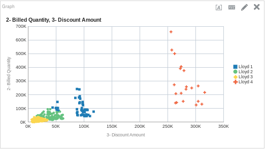
CLUSTER( ("Sales Person"."E0  Sales Rep Number", "Products"."P1  Product"), ("Base Facts"."2- Billed Quantity", "Base Facts"."3- Discount Amount"), 'clusterName', 'algorithm=k-means;method=Lloyd;numClusters=4;maxIter=12;useRandomSeed=TRUE;clusterNamePrefix=Lloyd')

And if we put that on a graph, it could look like this:

It works!

One More Time

Let’s do another example that shows the differences seen by adding or removing clusters. This time, let’s try out the Hierarchical cluster model. For this analysis, I want to see if there is a relationship between net costs and the average number of orders per sales rep (in Sample App 607, these are fact columns 17 and 24 respectively). Let’s start with three clusters to see what our data looks like. Here is the function, followed by the graph.

CLUSTER( ("Sales Person"."E0  Sales Rep Number", "Products"."P1  Product"), ("Simple Calculations"."17  Net Costs", "Simple Calculations"."24  Avg # of Orders by Sales Rep"), 'clusterName', 'algorithm=hierarchical;method=centroid;numClusters=3;maxIter=15;useRandomSeed=TRUE;clusterNamePrefix=Centroid')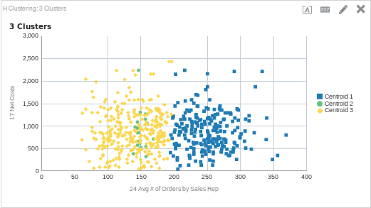

Barely three clusters in there!

To me, it seems that three clusters probably isn’t the right amount. Since both cluster 1 and 3 are so large (and cluster 2 so small), I would guess that if we add another cluster it could add some clarity as to what is happening here. Here is the same function with four clusters, along with the output.

CLUSTER( ("Sales Person"."E0  Sales Rep Number", "Products"."P1  Product"), ("Simple Calculations"."17  Net Costs", "Simple Calculations"."24  Avg # of Orders by Sales Rep"), 'clusterName', 'algorithm=hierarchical;method=centroid;numClusters=4;maxIter=15;useRandomSeed=TRUE;clusterNamePrefix=Centroid')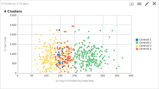

So… there is more to the picture!

After adding another cluster, we can see that there is another cluster between about 125 average orders to about 200 average orders (cluster 4). You may have noticed however, that there is still one large cluster that starts about 200 average orders and continues to the maximum number of average orders (cluster 2). What happens if we add another cluster?

CLUSTER( ("Sales Person"."E0  Sales Rep Number", "Products"."P1  Product"), ("Simple Calculations"."17  Net Costs", "Simple Calculations"."24  Avg # of Orders by Sales Rep"), 'clusterName', 'algorithm=hierarchical;method=centroid;numClusters=5;maxIter=15;useRandomSeed=TRUE;clusterNamePrefix=Centroid')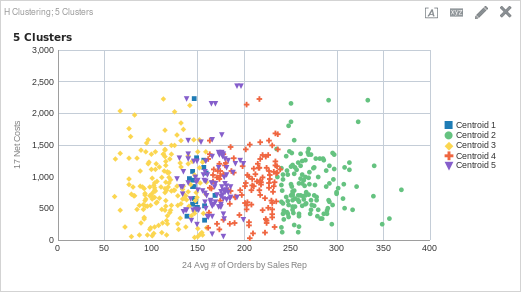

What is happening here?

What do you think? Is five clusters the right amount? Perhaps four? Is the algorithm the correct one? The thing about clustering is that even though we can use an algorithm to find similarities in the data and place like items into groups, it is still up to us to discover what the meaning is within the data set. This is as important as setting up the function and returning data. In my experience, the real work starts once the cluster function runs.

By looking at the above graphs, my initial reaction is that maybe this cluster analysis needs some more detail. Once the clusters are defined, I would create a table and start to add in more detail to see if there are any similarities. I would then try to incorporate these columns into the model, rerun, and see if there are any changes. It is also possible that I need to adjust my fact columns; maybe there is a better way to find relationships between those facts.

Doin’ It Right

Using the analytic functions in OBIEE is a paradigm shift in thinking for many OBIEE implementors and users; usually we build content that is easy to digest, reproducible and has a singular “right” answer. As we saw above, discovery and true analytics takes time and it takes critical thinking. This isn’t to say that clustering shouldn’t be on dashboards — dashboarding can be a powerful way to edit your clusters on the fly and enable discovery for more than just data analysts or scientists. And, I think once the function has been fine tuned to discover what each cluster means, content should be developed around those insights.

OBIEE and Analytics FTW