Almost always, joining fact tables is a big no-no in data modeling, and for good reason. From time to time however, we need to join fact tables because of architecture decisions that are outside of our control.

In this post I’ll tell you my method to the madness, and then we’ll see how to actually construct the solution in OBIEE 11g.
In Theory…
Recently I was asked to model a table that contained header level facts (we’ll call this HEADER_F) and another table that contained the detail level (we’ll call this DETAILS_F) to that fact table. Specifically, we need to create a metric that used two columns from the header level, and a column from detail level. Usually, we would see something like this when we have a star schema with conformed dimensions:
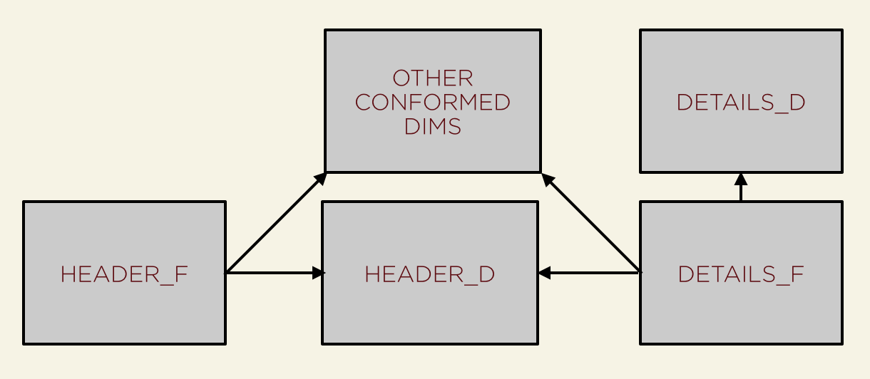
The Header Dim will become part of the conformed dimensional model, and should be joined to by the DETAILS_F. You’ll note that the DETAILS_D dimension is only joined to by the DETAILS_F table. This makes sense, since this is at a lower level of detail than the HEADER_F table. In this case, our Business Model in OBIEE would look the same as the physical layer; 1 Logical Table Source (LTS) per table and a beautiful constellation of joins. Nice to use, easy to model, and calculations are no problem at all due to the shared dimensions.
Now, what do you do if you don’t have a HEADER_D table? This could happen when all of the dimensionality has been moved into the fact table and are represented as what I like to call “Factributes”. These are the attribute and dimension columns that live within the fact table that should be within a dimension table. If an architecture decision has been made to have factributes within the fact table, then we have several options — either create an alias (or logical table) for the fact columns and an alias (or logical table) for the dimension columns, or leave it alone if we do not need that dimensionality. Not having a corresponding dimension table isn’t usually the case, but it does happen from time to time.
What happens if you also need to do calculations between the HEADER_F and DETAIL_F tables? Let’s pretend that we need to calculate a Net Amount logical column, and that this column is comprised of a Completed Amount, an Input Amount, and a Waste Amount. Let’s also imagine that two of these amounts are at the header level (Completed Amount and Waste Amount), and that one is at the detail level (Input Amount). To accomplish this, our Physical Model may look something more like this:
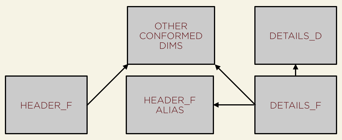
We could obviously join from DETAILS_F directly to HEADER_F, but by using an alias, we can keep the HEADER_F completely isolated from the DETAILS_F table, which will have query advantages (more on that below). This enables us to create a new logical table that has both the HEADER_F LTS and the joined HEADER_F alias and DETAILS_F LTS. This would look something like this:
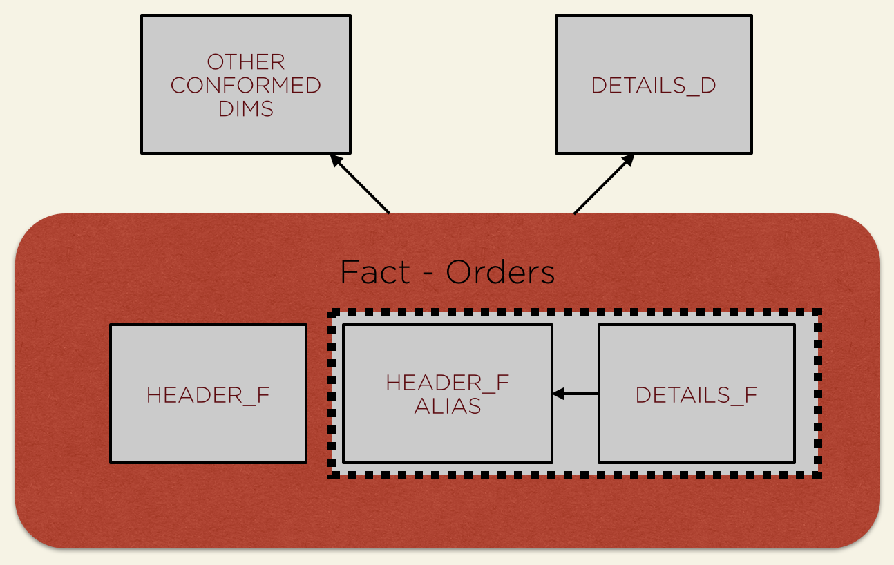
The biggest advantage to using this multiple logical table source approach is that we can now query HEADER_F alone for items that only reside in the HEADER_F table, or together with the DETAILS_F for the items in the DETAILS_F table. Since the Oracle BI Server will execute the join to the HEADER_F_ALIAS when we query the DETAILS_F table, we don’t need to worry about end users creating OBIEE Analysis that will result in an error (and who likes to get that “My report doesn’t work” email? Not me!). Also, if we only query for items in the DETAILS_F table, OBIEE will use “table pruning” and will not execute the join between the DETAILS_F and the HEADER_F_ALIAS tables.
Once we have the Logical Table created, we can easily create the logical measures for columns in HEADER_F, DETAIL_F, and our joint measure of (HEADER_F_ALIAS.COLUMN1 — DETAILS_F.COLUMN1— HEADER_F_ALIAS.COLUMN2).
In Practice…
Now that we have a conceptual understanding of what we are going to do, let’s put it to the test in OBIEE 11g.
First, let’s take a look at what the physical model could look like if we had a header dimension to join our two fact tables.
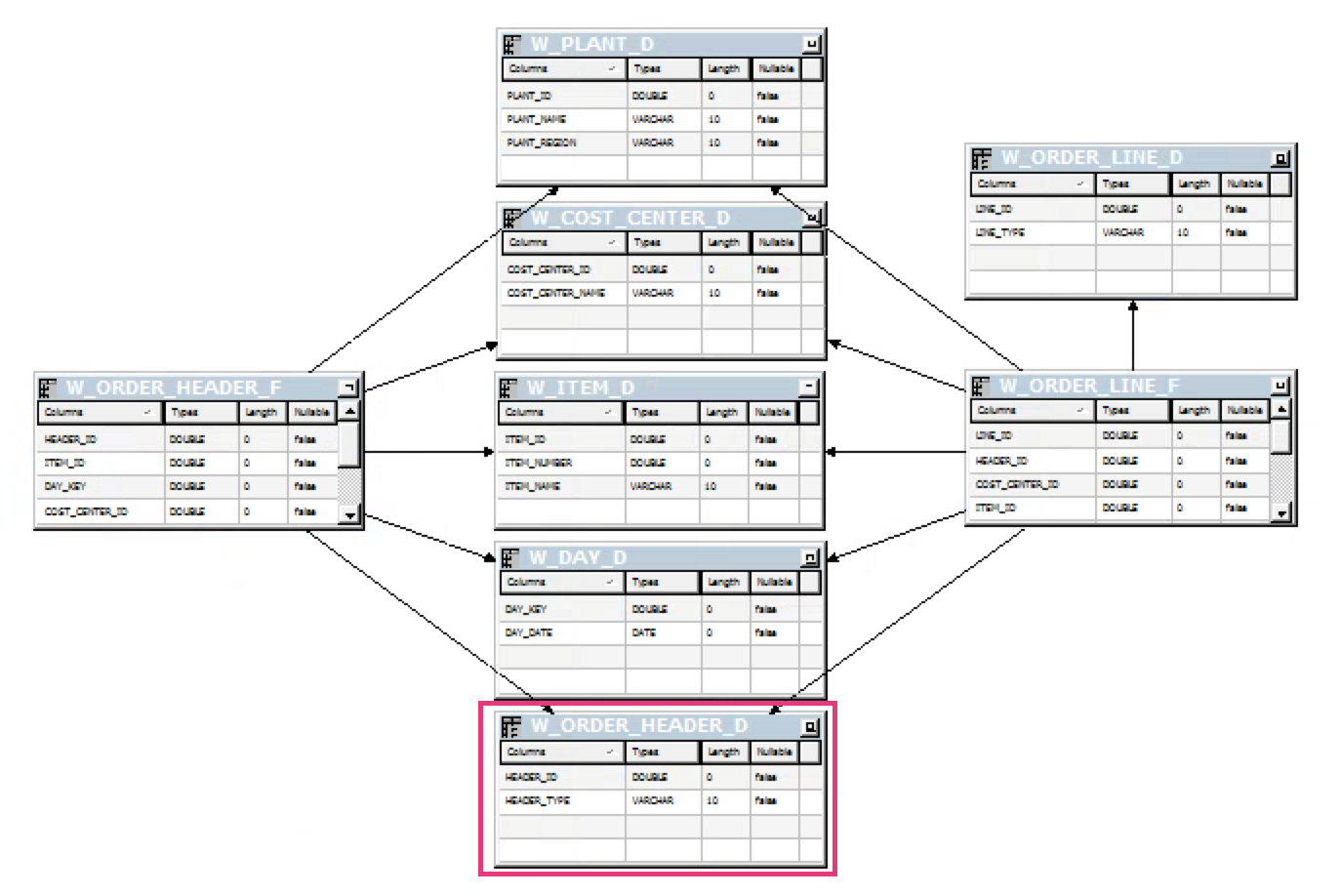
Like I said before, that isn’t the case in this scenario, so instead we have a physical model that looks like this (after we have created the header alias):
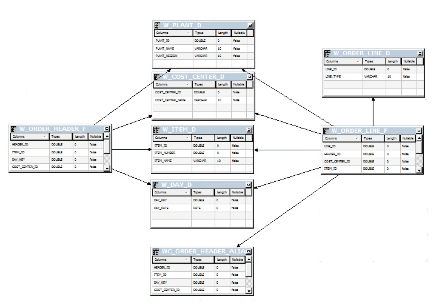
Now that we have our header fact aliased and joined to the details fact, let’s move on to the logical side of the house. As I discussed above, we’ll create two logical table sources. After creating a new logical table in the business model, create a new logical table source for the header fact. Mine looked like this:
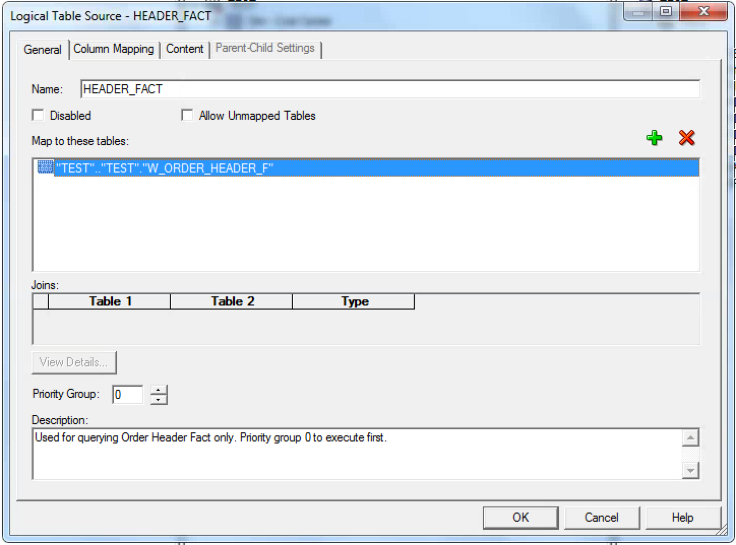
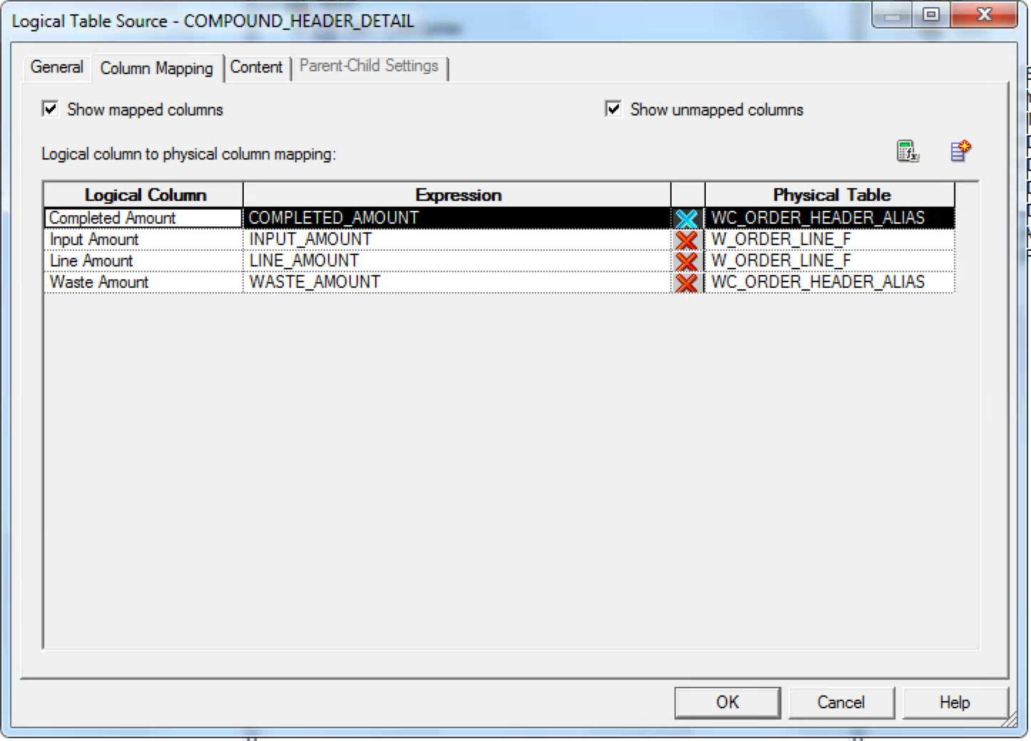
When creating this source, we’ll map all of the columns from W_HEADER_F in the content tab (like we usually would in this situation). Once we’re finished with W_HEADER_F, create another logical table source for the joined details and header alias tables (I called mine COMPOUND_HEADER_DETAIL). First add the details fact table, then followed by the aliased header table.
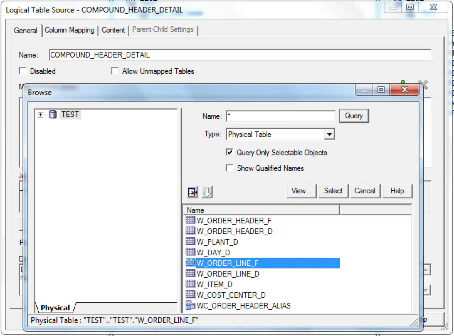
Next add the alias table to the to the logical table source. In my case, I used an inner join, although in some instances an outer may be applicable (an example of this may be in a scenario involving shipments and order lines). Also, be sure to change the Priority Group setting to “1”; this will execute the logical table source after the BI Server has already “checked” if other logical table source can answer the query call. Why is this advantageous? This reduces the cost of executing the query because the BI Server will not have to join the two facts each time if the query only requests items from the header fact. Pretty cool, huh?
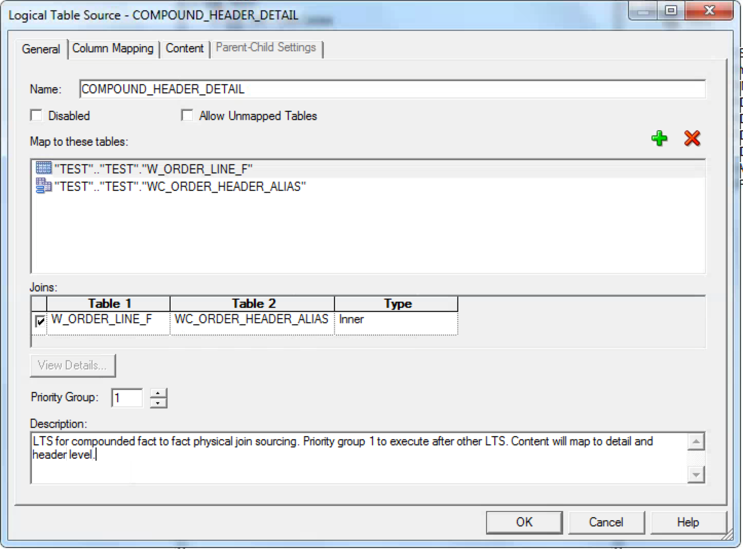
If we take a look at the content tab of the logical table source definition, we can map the header columns to the header alias, and the detail columns to the detail fact. This is important so that when we execute our measure (which we are soon to build), the BI Server will not think “You want to get columns from both Header and Details. I can go get the Header columns from the Header LTS.” This would defeat the entire purpose of joining the fact tables in our second logical table source. So, be sure to map those columns correctly!
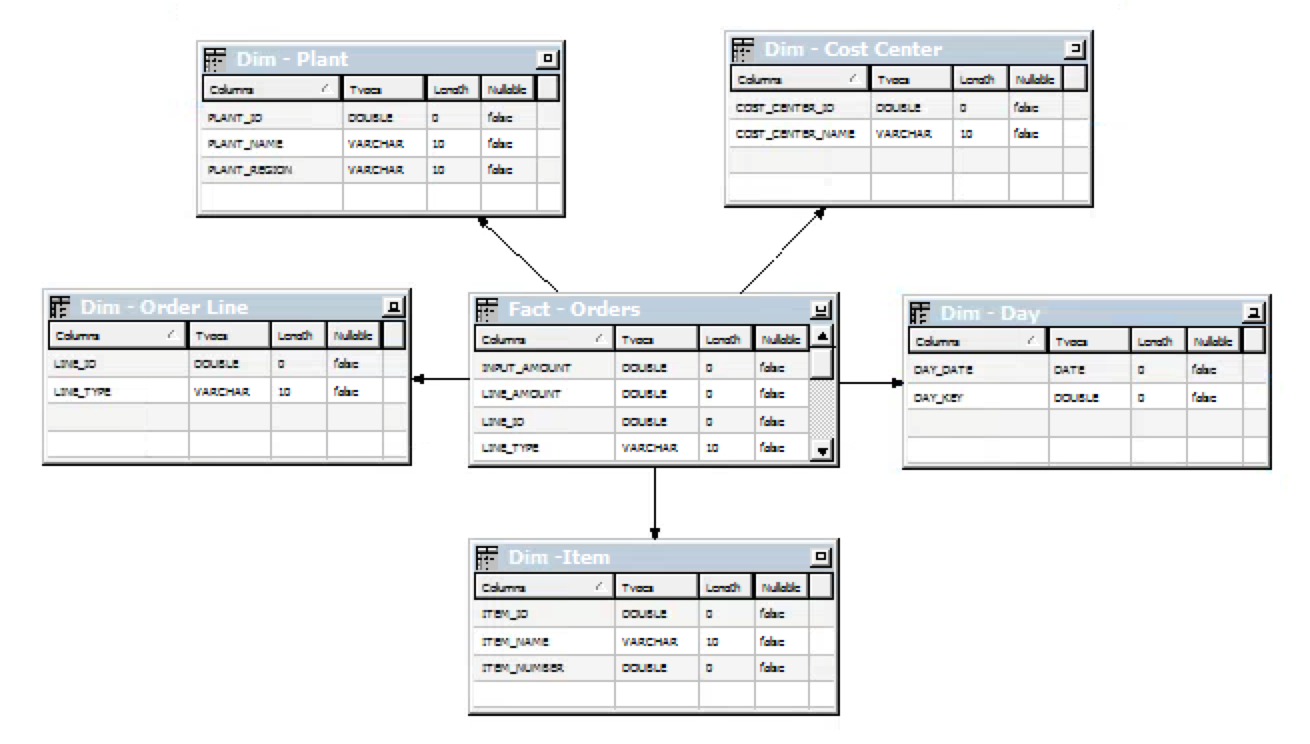
After we have mapped our columns, let’s take a look at our logical diagram. Since we joined the facts together and have multiple table sources, we’ll see one fact table instead of two fact tables with conformed dimensions between them (like we see in the physical layer).
Now that our columns are mapped and we have verified our logical fact diagram is correct, let’s create a new logical column. We’ll place the logic that we want for our calculated column in this new column. The logic in this example includes two columns from the alias table, and one from the detail fact. My column definition looked like this:
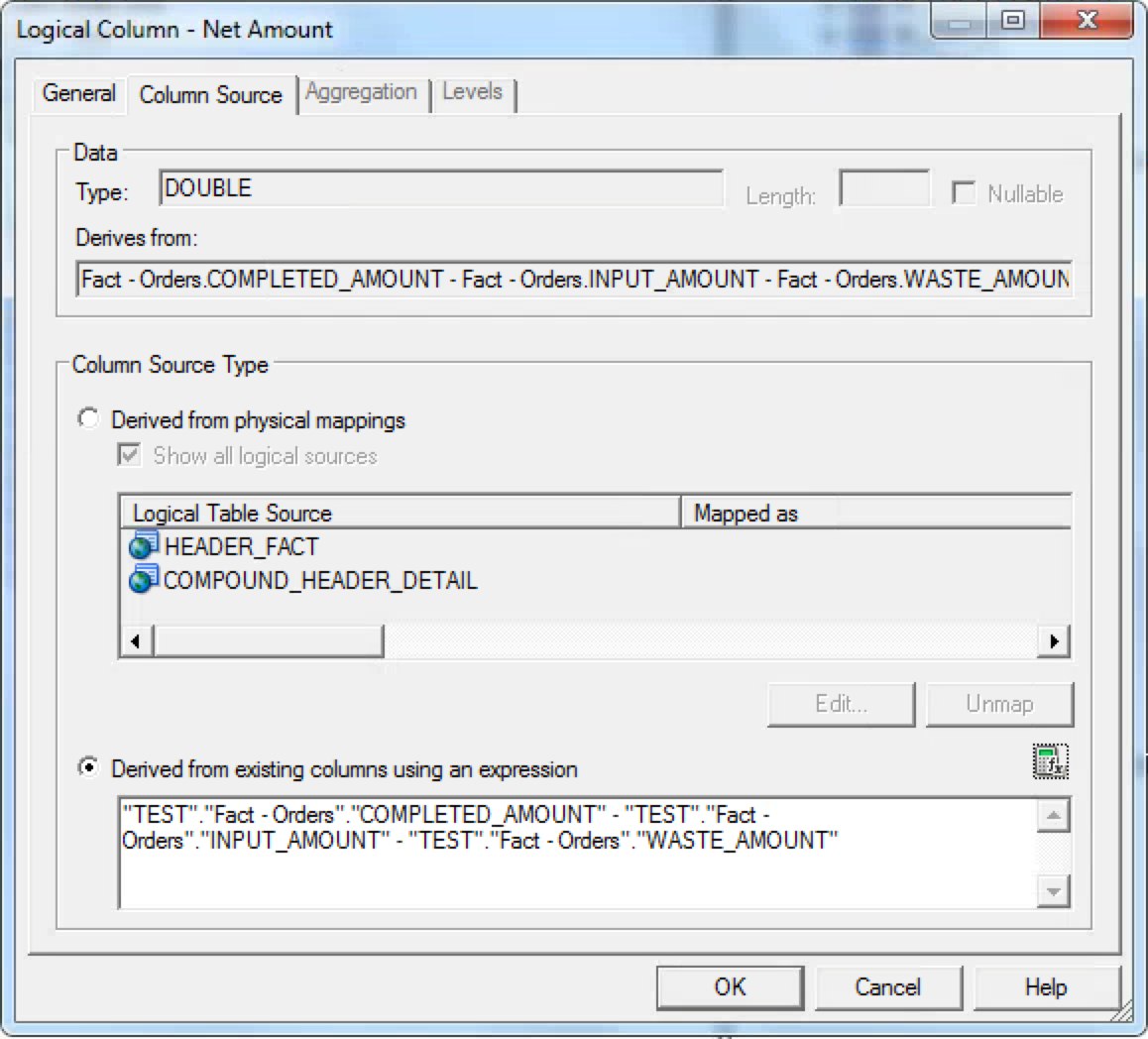
Since we mapped the logical COMPLETED_AMOUNT and WASTE_AMOUNT columns to the alias, when the column is executed it will use this mapping to resolve the column calculation, rather than using the header fact mapping. You may get a column symbol that looks like a dimension column with an “fx” on it; if so, make sure that your base measures have aggregation rules applied!

Now that we’ve finished the column, we should see something like this when we open our logical fact:
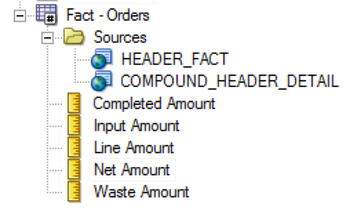
Now move the fact column(s) into your presentation layer and test the column.
In Conclusion…
Joining fact tables is never an ideal solution, but thankfully OBIEE 11g is equipped with the ability to allow us to navigate these situations. Using multiple table sources is a powerful tool, and one that can be leveraged to bring us accurate results for difficult query requests.