Employees at the Minneapolis Red Pill Analytics office recently had the luxury of sitting with Snowflake’s Steve Herskovitz for some on-site education. Among other things, one of my key takeaways from the exercise was how simple it is to query JSON data in the Snowflake Data Warehouse. The syntax is straightforward and makes the process of using JSON data in conjunction with relational data a relative breeze. In this post, I’ll walk through how to query JSON data and join it with a sample data set, make it readily available for a BI tool, and then display the results by connecting OBIEE and DV to the Snowflake Data Warehouse.
In preparation for this exercise, I have imported 2016 Week 1 NFL Kicking data to a spreadsheet and modified it slightly to add LAT/LON city coordinates and an indicator for whether the stadium is indoor or outdoor, in addition to the date/time the game started.
To get started, you have the option to run SQL statements from the Snowflake web UI, SnowSQL (CLI client), or a third-party tool such as SQL Developer or SQL Workbench/J; I’m using the web UI in this case. Throughout this post, I will intentionally leave out some of the details regarding basic navigation and functionality of Snowflake. The folks over at Snowflake have a pretty robust library of documentation here.
After logging in to Snowflake’s web UI, we need to create a table in a test database and insert the data containing statistics for all kickers with an attempt during week 1.
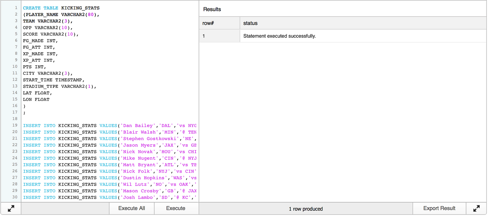
CREATE TABLE KICKING_STATS
 (PLAYER_NAME VARCHAR2(80),
 TEAM VARCHAR2(3),
 OPP VARCHAR2(10),
 SCORE VARCHAR2(10),
 FG_MADE INT,
 FG_ATT INT,
 XP_MADE INT,
 XP_ATT INT,
 PTS INT,
 CITY VARCHAR2(3),
 START_TIME TIMESTAMP,
 STADIUM_TYPE VARCHAR2(1),
 LAT FLOAT,
 LON FLOAT
 )
 ;
INSERT INTO KICKING_STATS VALUES('Blair Walsh','MIN','@ TEN','W 25-16','4','6','1','2','13','TEN','2016-09-11 12:00:00','O',36.16589,-86.784439);
INSERT INTO KICKING_STATS VALUES('Stephen Gostkowski','NE','@ ARI','W 23-21','3','3','2','2','11','ARI','2016-09-11 19:30:00','I',33.44838,-112.074043);
INSERT INTO KICKING_STATS VALUES('Jason Myers','JAX','vs GB','L 23-27','3','3','2','2','11','JAX','2016-09-11 12:00:00','O',30.33218,-81.655647);
INSERT INTO KICKING_STATS VALUES('Nick Novak','HOU','vs CHI','W 23-14','3','3','2','2','11','HOU','2016-09-11 12:00:00','I',29.763281,-95.363274);
INSERT INTO KICKING_STATS VALUES('Mike Nugent','CIN','@ NYJ','W 23-22','3','4','2','2','11','NYJ','2016-09-11 12:00:00','O',43.000351,-75.499901);
INSERT INTO KICKING_STATS VALUES('Matt Bryant','ATL','vs TB','L 24-31','3','3','1','1','10','ATL','2016-09-11 12:00:00','I',33.749001,-84.387978);
INSERT INTO KICKING_STATS VALUES('Nick Folk','NYJ','vs CIN','L 22-23','3','4','1','2','10','NYJ','2016-09-11 12:00:00','O',43.000351,-75.499901);
INSERT INTO KICKING_STATS VALUES('Dustin Hopkins','WAS','vs PIT','L 16-38','3','3','1','1','10','WAS','2016-09-12 18:10:00','O',38.895111,-77.036369);
INSERT INTO KICKING_STATS VALUES('Wil Lutz','NO','vs OAK','L 34-35','2','4','4','4','10','NO','2016-09-11 12:00:00','I',29.954651,-90.075073);
INSERT INTO KICKING_STATS VALUES('Mason Crosby','GB','@ JAX','W 27-23','2','2','3','3','9','JAX','2016-09-11 12:00:00','O',30.33218,-81.655647);
INSERT INTO KICKING_STATS VALUES('Josh Lambo','SD','@ KC','L 27-33','2','3','3','3','9','KC','2016-09-11 12:00:00','O',39.099731,-94.578568);
INSERT INTO KICKING_STATS VALUES('Cairo Santos','KC','vs SD','W 33-27','2','2','3','3','9','KC','2016-09-11 12:00:00','O',39.099731,-94.578568);
INSERT INTO KICKING_STATS VALUES('Caleb Sturgis','PHI','vs CLE','W 29-10','2','3','3','3','9','PHI','2016-09-11 12:00:00','O',39.952339,-75.163788);
INSERT INTO KICKING_STATS VALUES('Adam Vinatieri','IND','vs DET','L 35-39','2','2','3','3','9','IND','2016-09-11 15:25:00','I',39.768379,-86.158043);
INSERT INTO KICKING_STATS VALUES('Chris Boswell','PIT','@ WAS','W 38-16','1','1','5','5','8','WAS','2016-09-12 18:10:00','O',38.895111,-77.036369);
INSERT INTO KICKING_STATS VALUES('Graham Gano','CAR','@ DEN','L 20-21','2','3','2','2','8','DEN','2016-09-08 19:30:00','O',39.739151,-104.984703);
INSERT INTO KICKING_STATS VALUES('Roberto Aguayo','TB','@ ATL','W 31-24','1','1','4','4','7','ATL','2016-09-11 12:00:00','I',33.749001,-84.387978);
INSERT INTO KICKING_STATS VALUES('Sebastian Janikowski','OAK','@ NO','W 35-34','2','2','1','1','7','NO','2016-09-11 12:00:00','I',29.954651,-90.075073);
INSERT INTO KICKING_STATS VALUES('Matt Prater','DET','@ IND','W 39-35','1','1','4','5','7','IND','2016-09-11 15:25:00','I',39.768379,-86.158043);
INSERT INTO KICKING_STATS VALUES('Justin Tucker','BAL','vs BUF','W 13-7','2','2','1','1','7','BAL','2016-09-11 12:00:00','O',39.290379,-76.61219);
INSERT INTO KICKING_STATS VALUES('Steven Hauschka','SEA','vs MIA','W 12-10','2','2','0','1','6','SEA','2016-09-11 15:05:00','O',47.606209,-122.332069);
INSERT INTO KICKING_STATS VALUES('Phil Dawson','SF','vs LA','W 28-0','0','0','4','4','4','SF','2016-09-12 21:20:00','O',37.774929,-122.419418);
INSERT INTO KICKING_STATS VALUES('Andrew Franks','MIA','@ SEA','L 10-12','1','2','1','1','4','SEA','2016-09-11 15:05:00','O',47.606209,-122.332069);
INSERT INTO KICKING_STATS VALUES('Patrick Murray','CLE','@ PHI','L 10-29','1','1','1','1','4','PHI','2016-09-11 12:00:00','O',39.952339,-75.163788);
INSERT INTO KICKING_STATS VALUES('Ryan Succop','TEN','vs MIN','L 16-25','1','1','1','1','4','TEN','2016-09-11 12:00:00','O',36.16589,-86.784439);
INSERT INTO KICKING_STATS VALUES('Chandler Catanzaro','ARI','vs NE','L 21-23','0','1','3','3','3','ARI','2016-09-11 19:30:00','I',33.44838,-112.074043);
INSERT INTO KICKING_STATS VALUES('Brandon McManus','DEN','vs CAR','W 21-20','0','0','3','3','3','DEN','2016-09-08 19:30:00','O',39.739151,-104.984703);
INSERT INTO KICKING_STATS VALUES('Connor Barth','CHI','@ HOU','L 14-23','0','0','2','2','2','HOU','2016-09-11 12:00:00','I',29.763281,-95.363274);
INSERT INTO KICKING_STATS VALUES('Randy Bullock','NYG','@ DAL','W 20-19','0','0','2','3','2','DAL','2016-09-11 15:25:00','I',32.783058,-96.806671);
INSERT INTO KICKING_STATS VALUES('Dan Carpenter','BUF','@ BAL','L 7-13','0','1','1','1','1','BAL','2016-09-11 12:00:00','O',39.290379,-76.61219);
COMMIT;
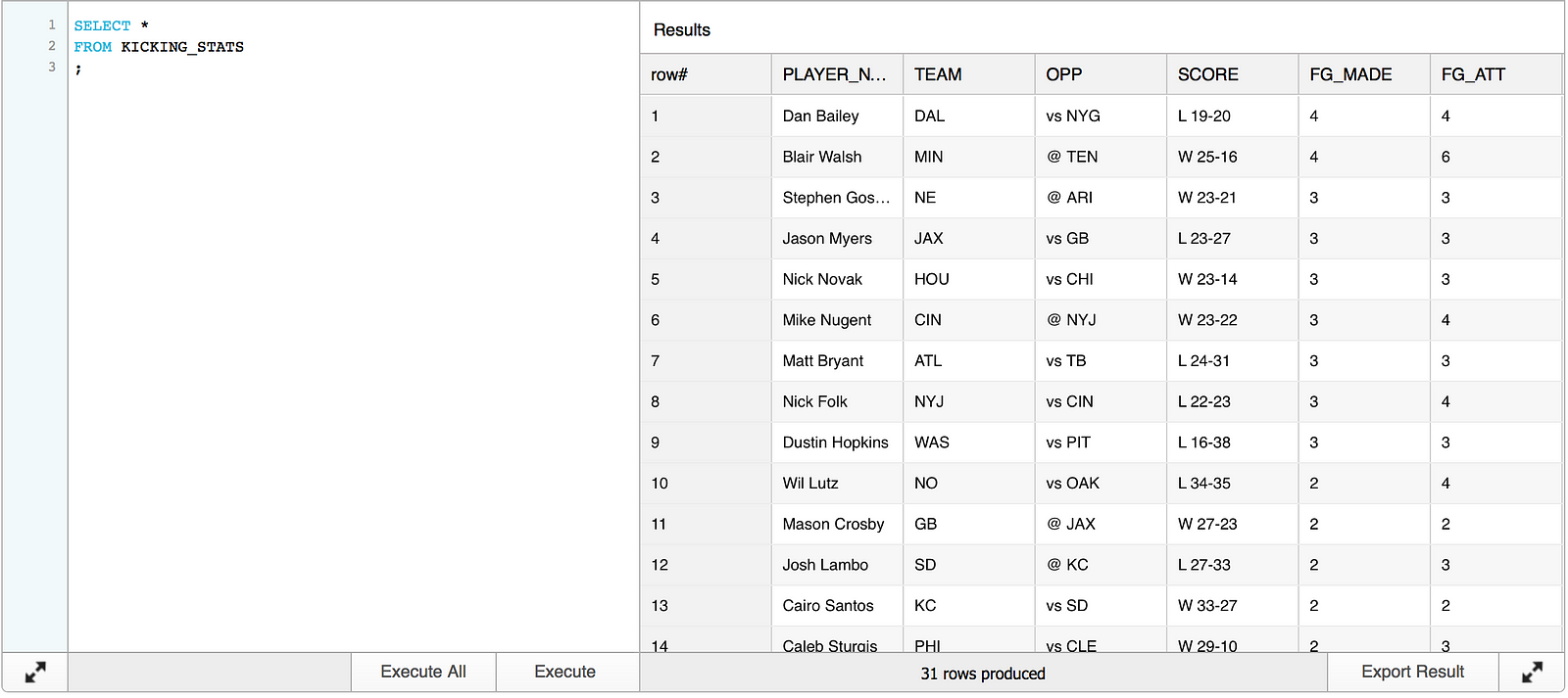
Select * shows that the table was created and is populated with data:
Let’s move on to the JSON data.
Snowflake has added a database named SNOWFLAKE_SAMPLE_DATA that contains public weather data, among a handful of other sample data sets. The weather data is sourced from http://www.openweathermap.com.
Running the SHOW TABLES command in the SNOWFLAKE_SAMPLE_DATA database reveals five sample weather data tables.
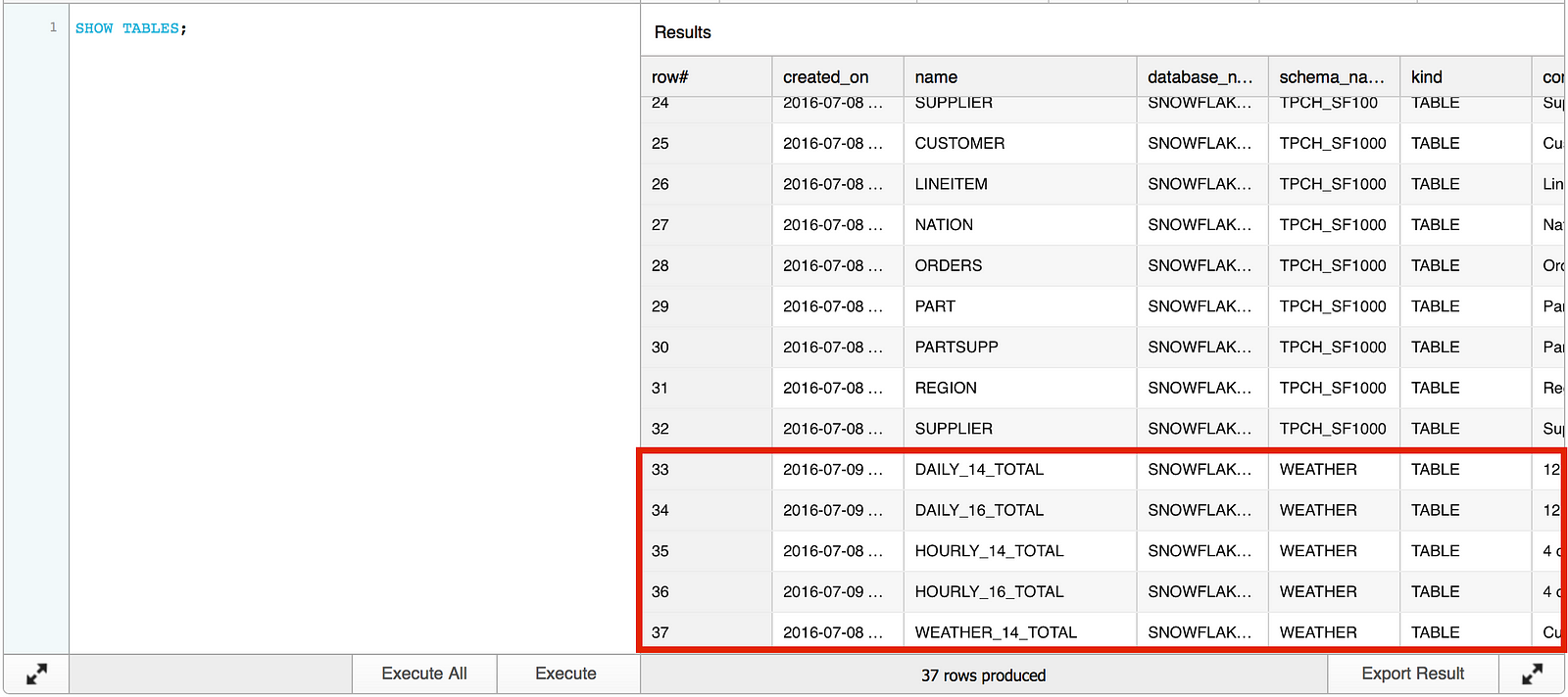
Information regarding the data these tables contain can be found here. We are going to use the WEATHER_14_TOTAL table, which contains hourly weather data for 20,000 cities.
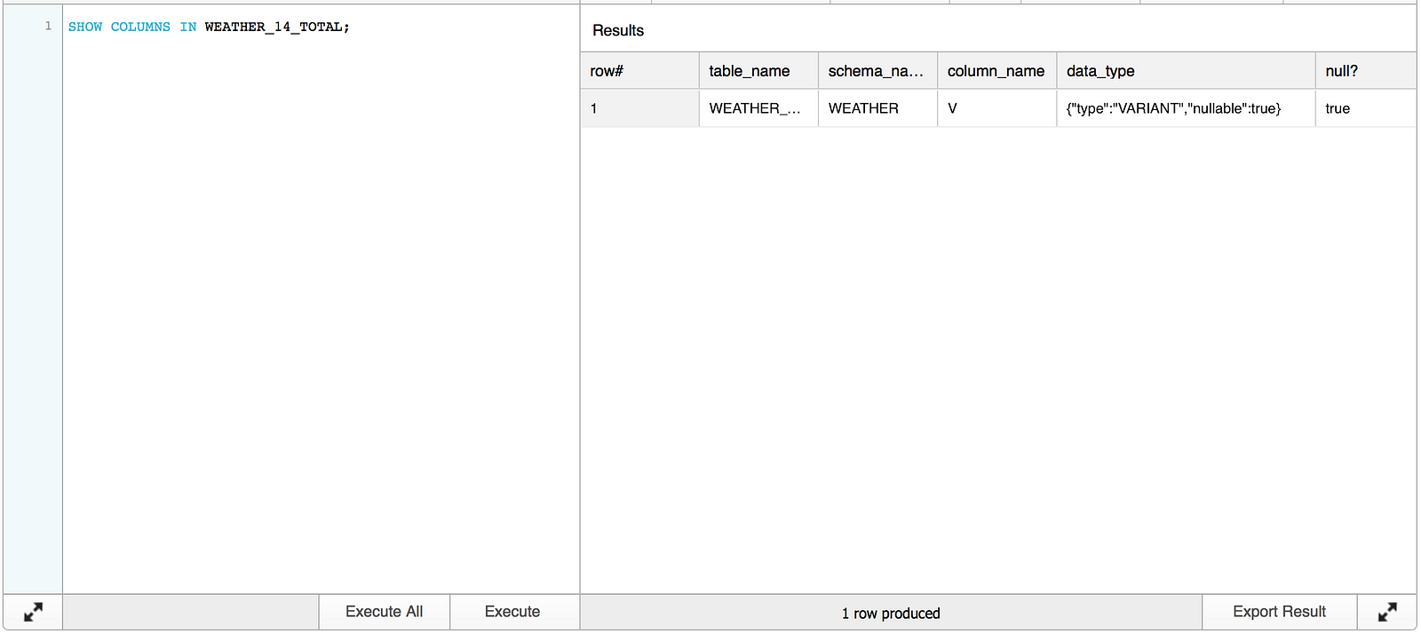
Let’s have a look at the data in WEATHER_14_TOTAL. Running the SHOW COLUMNS command for WEATHER_14_TOTAL returns one column named V with a VARIANT data type.
A simple select against the table shows that V contains a hyperlinked data set.
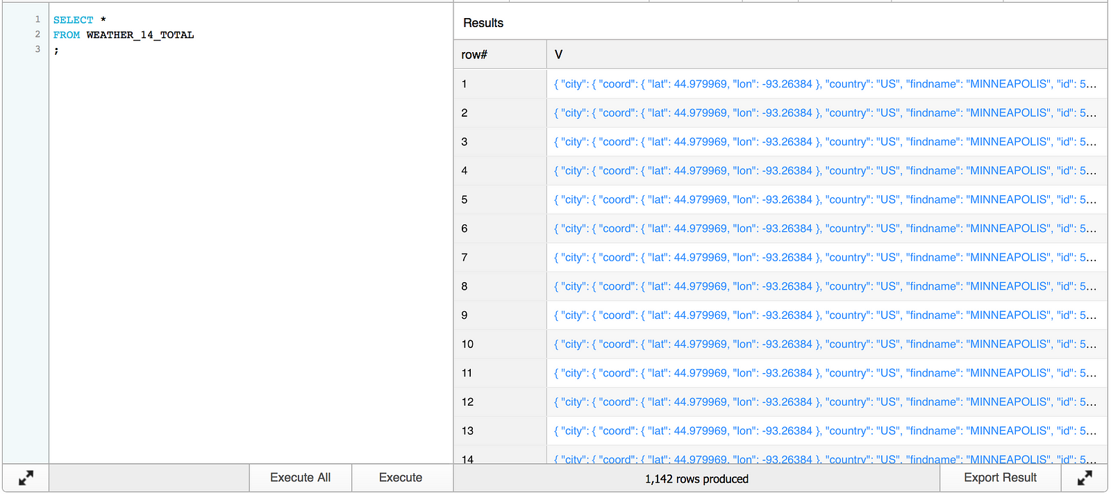
Clicking on one of the hyperlinks reveals JSON data. For example, an entry for Minneapolis, MN, USA looks something like this:
{
 “city”: {
 “coord”: {
 “lat”: 44.979969,
 “lon”: -93.26384
 },
 “country”: “US”,
 “findname”: “MINNEAPOLIS”,
 “id”: 5037649,
 “langs”: [
 {
 “bg”: “Минеаполис”
 },
 {
 “ca”: “Minneapolis”
 },
 {
 “da”: “Minneapolis”
 },
 {
 “de”: “Minneapolis”
 },
 {
 “en”: “Minneapolis”
 },
 {
 “eo”: “Minneapolis”
 },
 {
 “es”: “Minneapolis”
 },
 {
 “fi”: “Minneapolis”
 },
 {
 “fr”: “Minneapolis”
 },
 {
 “ga”: “Minneapolis”
 },
 {
 “gl”: “Minneapolis”
 },
 {
 “he”: “מיניאפוליס”
 },
 {
 “hu”: “Minneapolis”
 },
 {
 “id”: “Minneapolis”
 },
 {
 “io”: “Minneapolis”
 },
 {
 “it”: “Minneapolis”
 },
 {
 “ja”: “ミネアポリス”
 },
 {
 “la”: “Minneapolis”
 },
 {
 “link”: “http://en.wikipedia.org/wiki/Minneapolis”
 },
 {
 “mr”: “मिनीआपोलिस”
 },
 {
 “nl”: “Minneapolis”
 },
 {
 “nn”: “Minneapolis”
 },
 {
 “no”: “Minneapolis”
 },
 {
 “pl”: “Minneapolis”
 },
 {
 “post”: “55447”
 },
 {
 “pt”: “Minneapolis”
 },
 {
 “ru”: “Миннеаполис”
 },
 {
 “sk”: “Minneapolis”
 },
 {
 “sv”: “Minneapolis”
 },
 {
 “tr”: “Minneapolis”
 },
 {
 “zh”: “明尼阿波利斯”
 }
 ],
 “name”: “Minneapolis”,
 “zoom”: 5
 },
 “clouds”: {
 “all”: 40
 },
 “main”: {
 “humidity”: 94,
 “pressure”: 1009,
 “temp”: 293.22,
 “temp_max”: 295.15,
 “temp_min”: 291.15
 },
 “time”: 1473325242,
 “weather”: [
 {
 “description”: “scattered clouds”,
 “icon”: “03n”,
 “id”: 802,
 “main”: “Clouds”
 }
 ],
 “wind”: {
 “deg”: 250,
 “speed”: 3.1
 }
}
To query this JSON data set in Snowflake, simply tell the query to navigate the levels of the JSON record and filter on the values at each level. For example, to query for country = US and city = Minneapolis, execute the following query:
SELECT *
FROM WEATHER_14_TOTAL
WHERE v:city:country = 'US'
AND v:city:name = 'Minneapolis'
;
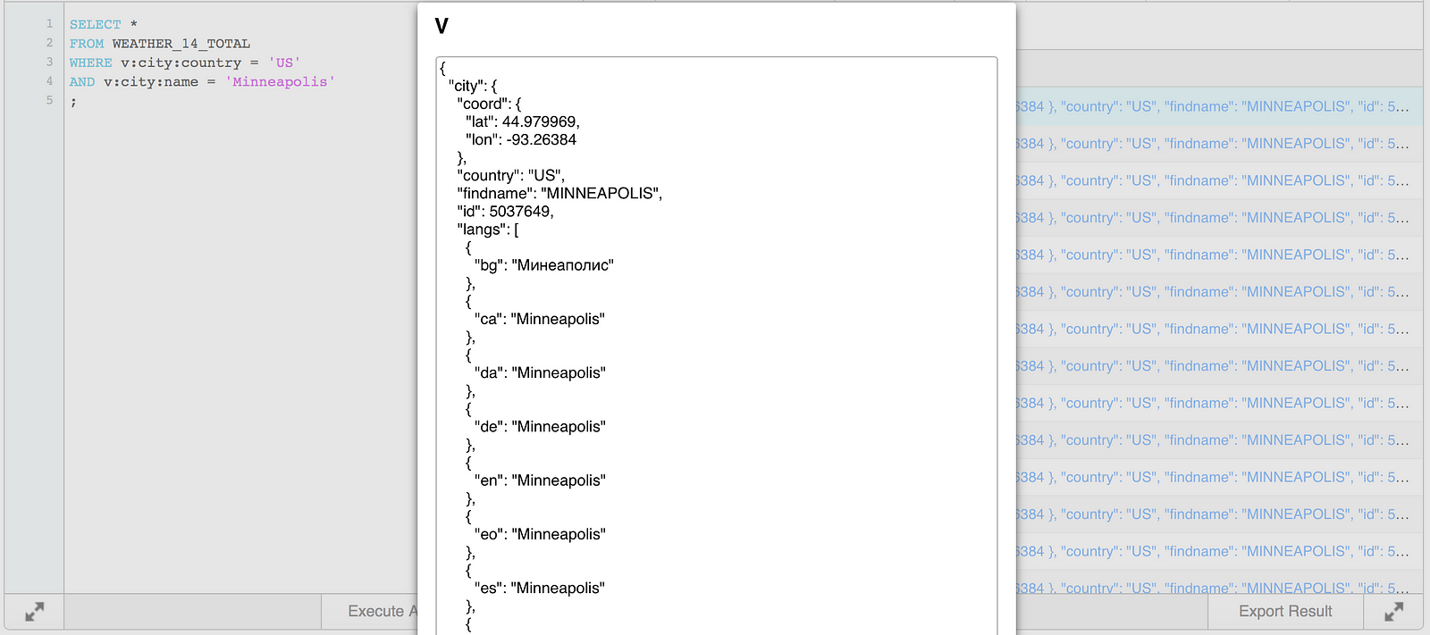
Going back to the data loaded in KICKING_STATS, LAT and LON values are available to use in place of country/city name. In the JSON record, LAT and LON are stored in city:coord:lat and city:coord:lon, respectively.
The JSON file also contains a timestamp, stored in unix time. We can translate unix time to a timestamp using the to_timestamp_ltz() function which will convert to the local timestamp (I’ve set my session to be in US Central time). We can now include this timestamp in the join to KICKING_STATS on game start time.
Disclaimer: This post is not meant to be a true analysis of NFL kicking performance. It does not contain key information on variables such as wind direction, actual speed at time of kick, etc. — I’ll make sure any feedback regarding the topic makes it to the suggestion box:

The SQL below joins the KICKING_STATS table to the sample weather data on LAT/LON and the max timestamp prior to each game’s start time. The results will include all of the data in KICKING_STATS as well as the temperature and wind speed from WEATHER_14_TOTAL. Temperature is stored in kelvin and wind speed in meters per second; I’ve chosen to use some basic arithmetic to convert temperature to fahrenheit and wind speed to miles per hour. To reiterate, the resulting data will not contain all of the specifics we need to do useful analytics but it will give a general idea of weather conditions when the game started.
SELECT (B.v:main:temp*(9/5))-459.67 AS TEMP_F,
 B.v:wind:speed*2.23694 AS WIND_MPH,
 A.*
FROM KICKING_STATS A,
 SNOWFLAKE_SAMPLE_DATA.WEATHER.WEATHER_14_TOTAL B
WHERE 1=1
AND A.LAT = B.v:city:coord:lat
AND A.LON = B.v:city:coord:lon
AND B.v:time = (SELECT MAX(C.v:time) FROM SNOWFLAKE_SAMPLE_DATA.WEATHER.WEATHER_14_TOTAL C
 WHERE A.LAT = C.v:city:coord:lat
 AND A.LON = C.v:city:coord:lon
 AND TO_TIMESTAMP_LTZ(C.v:time) <= A.START_TIME)
;
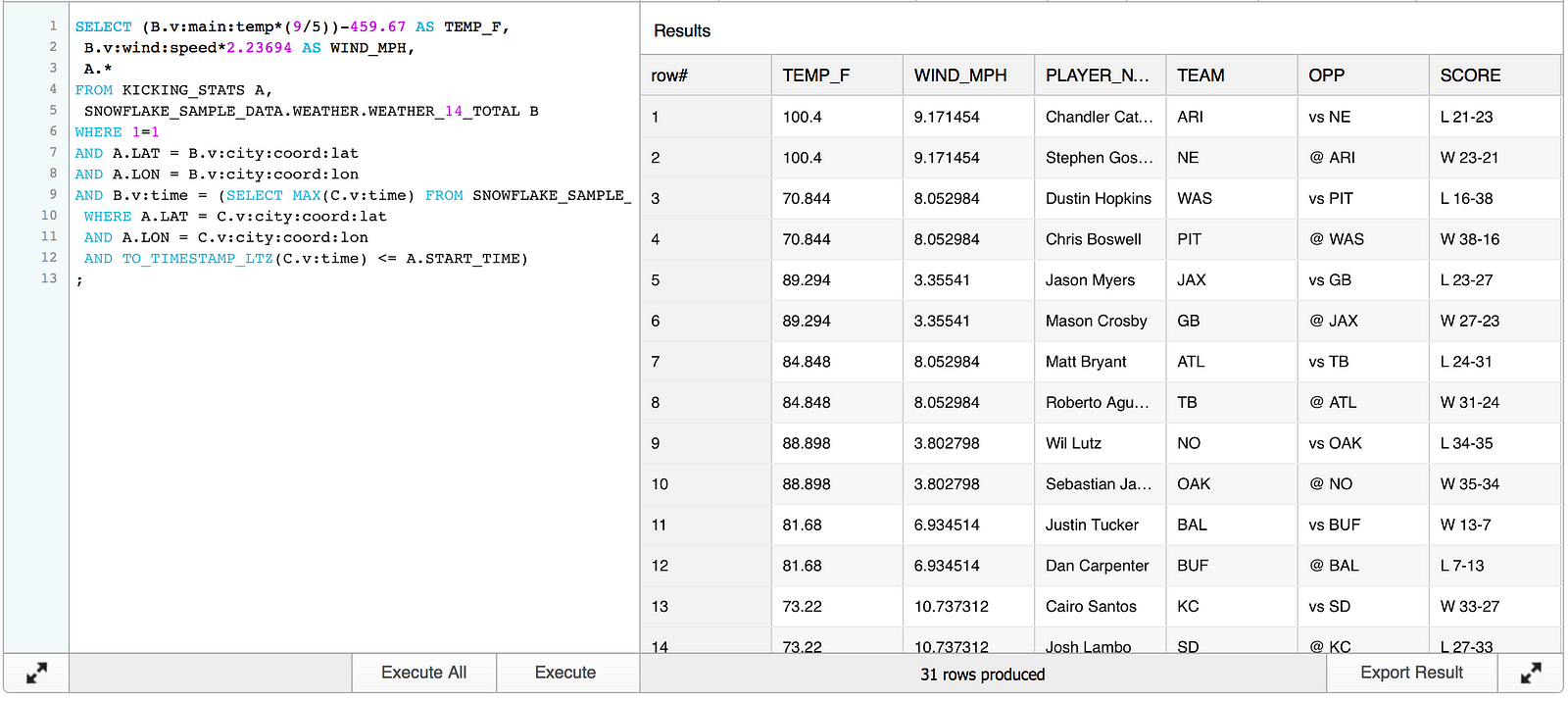
Stopping right there demonstrates some pretty cool technology. Again, there is quite a bit of useful information on the Snowflake website detailing how to query and flatten JSON data. One good reference is a blog post by Saqib Mustafa and Kent Graziano.
Now let’s take it another step and make the data easily available for a BI tool and display the results using OBIEE. Creating a view for the query from above will simplify the process for reuse in OBIEE.
CREATE OR REPLACE VIEW OBI_KICKING_STATS (PLAYER_NAME,TEAM,OPP,SCORE,FG_MADE,FG_ATT,XP_MADE,XP_ATT,PTS,CITY,START_TIME,STADIUM_TYPE,LAT,LON,TEMP_F,WIND_MPH)
AS (SELECT A.*,
 (B.v:main:temp*(9/5))-459.67 AS TEMP_F,
  B.v:wind:speed*2.23694 AS WIND_MPH
FROM KICKING_STATS A,
  SNOWFLAKE_SAMPLE_DATA.WEATHER.WEATHER_14_TOTAL B
WHERE 1=1
AND A.LAT = B.v:city:coord:lat
AND A.LON = B.v:city:coord:lon
AND B.v:time = (SELECT MAX(C.v:time) FROM SNOWFLAKE_SAMPLE_DATA.WEATHER.WEATHER_14_TOTAL C
 WHERE A.LAT = C.v:city:coord:lat
 AND A.LON = C.v:city:coord:lon
 AND TO_TIMESTAMP_LTZ(C.v:time) <= A.START_TIME)
 )
 ;
With the view created, OBIEE needs a Snowflake connection. I have downloaded the Snowflake ODBC driver and set up a new connection by following Phil’s instructions to connect OBIEE to Snowflake. Now that the setup is complete, we need to bring in the view from Snowflake as a physical source in OBIEE and configure the metadata:
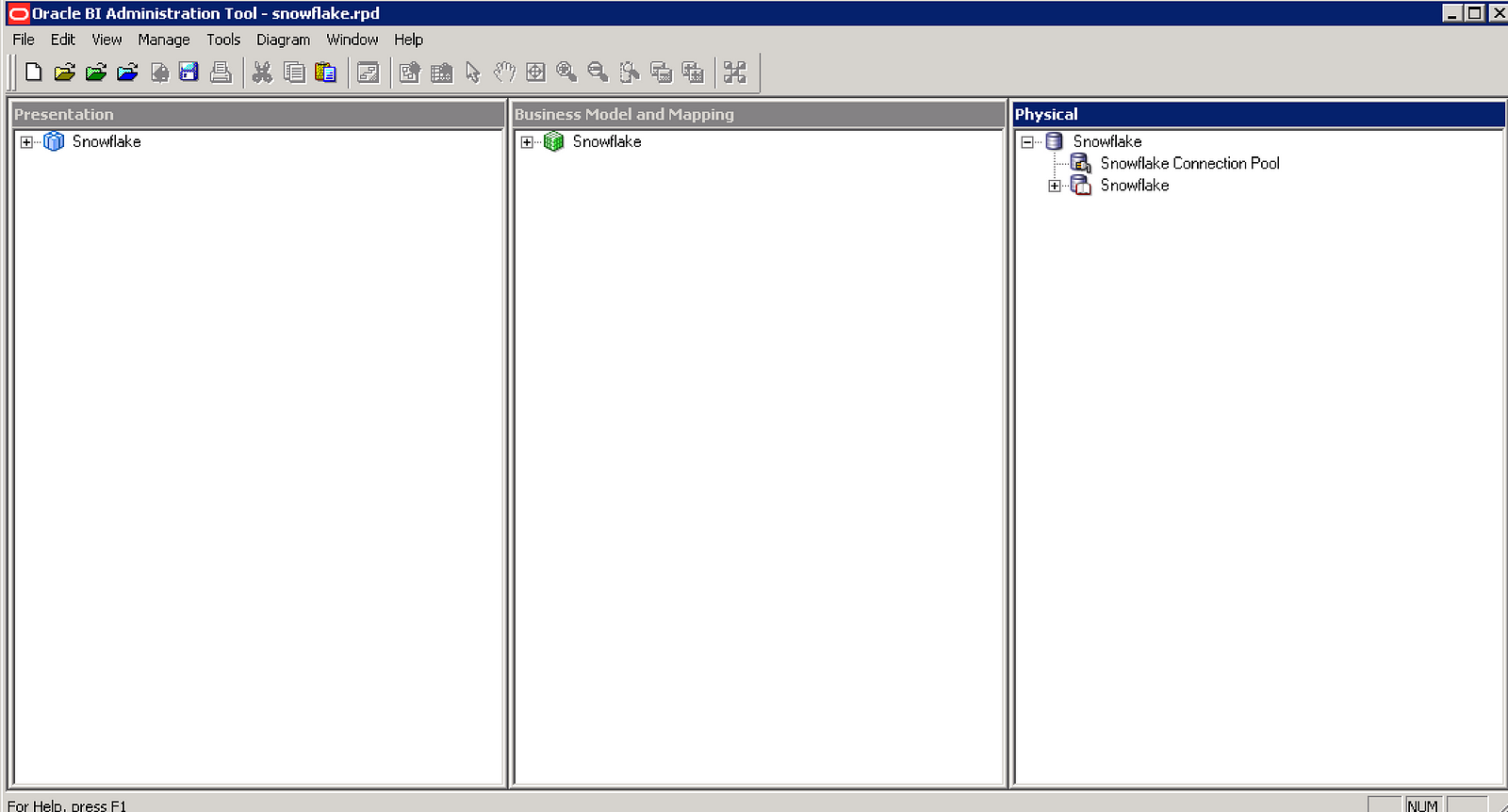
After deploying snowflake.rpd and restarting the services, let’s create a basic report and display the results in a table to check that the connection works and data is flowing through.
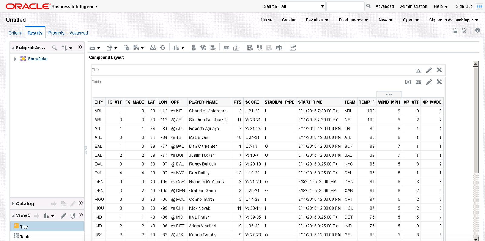
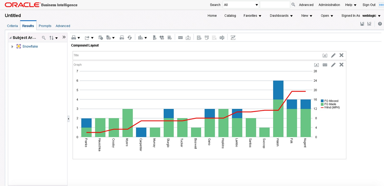
Fantastic! The query is successful and the data from Snowflake displays in an OBIEE analysis but since Oracle has a newer car in the garage, it may as well be taken out for a test drive. In OBIEE 12c (and some versions of OBIEE 11g), reports and visualizations in Oracle DV can be written against OBIEE subject areas.
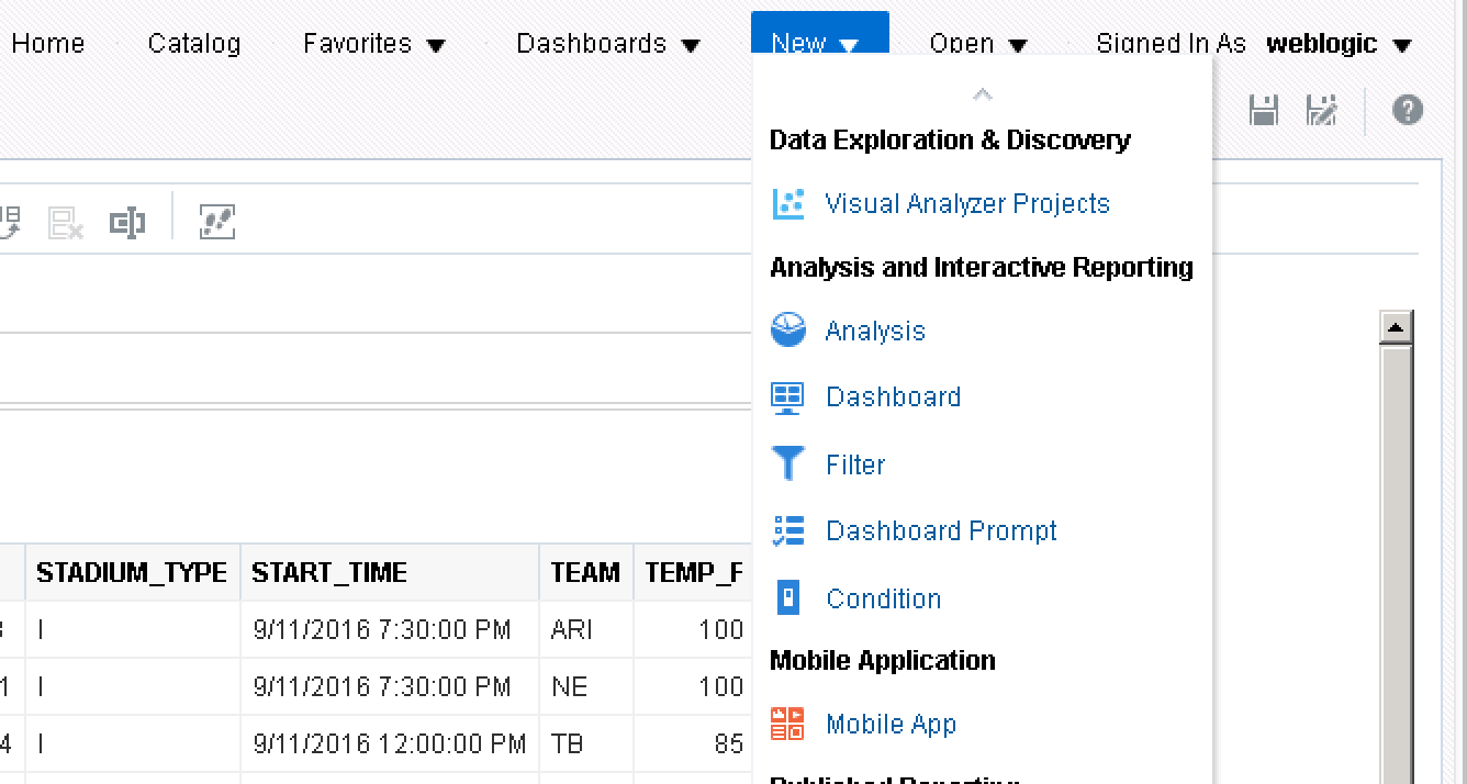
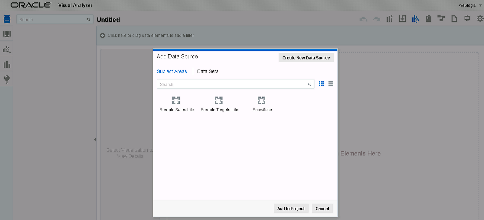
We can create a visualization in DV by using the Snowflake subject area from the metadata and front-end screen captures shown above. I created a calculated metric for extra-point percent (extra-points made/extra-point attempts) and used it to help build a visualization with the data from the view.
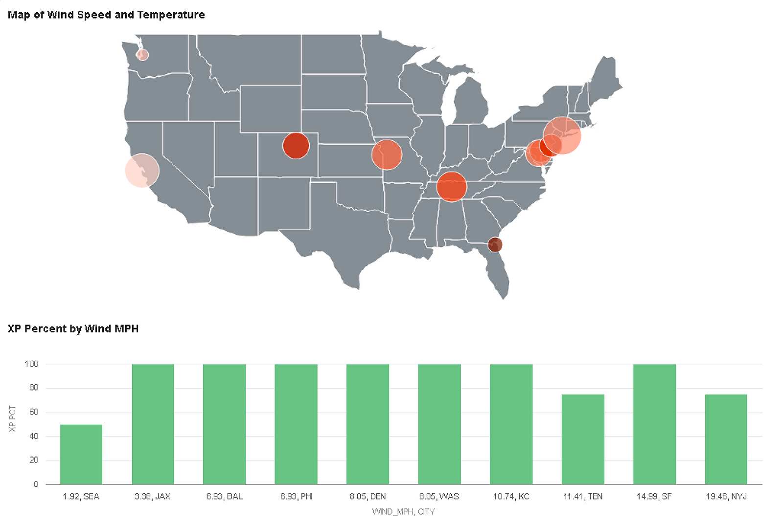
That’s it. With some SQL and basic OBIEE configuration, we were able to display a map of temperature and wind speed stored in JSON in the Snowflake Data Warehouse and combine the JSON data with some curated relational data to display a few charts. This is impressive given there wasn’t any data movement nor parsing of files; the true source of the weather data shown above is JSON data stored in a column with a variant data type.