I think it’s fair to say that I like models. Whether manifested with Legos, metadata, or economic indicators, I love seeing how inputs can affect outputs. So, when I discovered the forecast capabilities in the R suite, I couldn’t wait to give it a go.
Never Tell Me the Odds!
Many of the companies I have worked with either as a full time employee or as a consultant have struggled with forecasting. Without the proper toolset it can be difficult to accurately project where sales, inventory, or orders may be in the future. 12c’s Forecast function can take away many of the pain points associated with forecasting: poor data, lack of data, lack of statistical skill, and lack of time. For those skeptics out there, why wouldn’t you want to know what is within the realm of possibility (statistically speaking) based on past trends? Below we’ll walk through some examples of how this function works, and what options and parameters are available.

Feel the Forecast
Let’s take a look at the syntax on the Forecast function, and then I’ll break down the options and parameters.
FORECAST(numeric_expr, ([series]), output_column_name, options, [runtime_binded_options] )
Looks simple, and we even have the benefit of several optional parameters. What does each mean? I’m glad you asked…
numeric_expr is the metric that you wish to forecast.
series is an optional parameter that dictates the grain of the date/time dimension on which the forecast will be conducted. This can be a series of date/time dimension columns, or just a singular input, depending on how you’d like to forecast. If this parameter is omitted, the BI server will determine the level of the time dimension to use at run time. (A quick digression on this topic: make sure you have a properly configured time dimension with a working hierarchy to prevent the BI Server from getting confused. Also, be sure to set this column if your selected measure column joins to multiple date/time dimensions!)
output_column_name is the type of forecast that will be run. The valid options here are ‘forecast’, ‘low’, ‘high’ and ‘predictionInterval’. Each option will slightly change the forecasted values. As you may have guessed, ‘low’and ‘high’ show the lower and upper bounds of the forecast output, respectively. The ‘forecast’ option will display the result of the forecast; unless you specify a prediction interval (as seen in a different option below), the default will be 95% confidence. Lastly, the ‘predictionInterval’ column shows the prediction interval level used in the forecast.
options are additional parameters that can be specified for the function. The entire options set should be contained in single quotations, and separated with semi-colons (see examples below). These options can equal variables as well; presentation variables or the run-time options are acceptable. To use the run-time options, set the option to %1…%N. The number following the percentage sign indicates the number of the option in the list of run-time variables. There will be examples below, so don’t fret if this isn’t making sense at the moment.
There are many different inputs available for the forecast functions optionsparameter. Let’s walk through them.
The ‘numPeriods’ option specifies the number of periods to run the forecast. Each period is one unit of the lowest level grain you have selected for the series option described above. This value is an integer.
‘predictionInterval’ determines the level of confidence of the forecast. This is a value between 0 and 100, where 0 is the lower bound and 100 is the upper bound of the forecast. As I stated above, the default if 95% if this option is omitted.
The ‘modelType’ parameter selects the model to use for the forecast. There are two acceptable values for this parameter: ‘arima’ and ‘ets’. There literally have been books written about different forecasting models, so I will try to succinctly describe the two options here. ARIMA stands for Autoregressive Integrated Moving Average. What this means in layperson’s terms is that the model will regress values over a time series, smooth errors linearly, and replace data points with the delta between points. The goal is to smooth the data and create an output that fits the data as well as possible. ETS on the other hand, stands for Error, Trend, Seasonality and is an exponential smoothing model. This type allows for more fine tuning of the model by parameterizing specific model simulations. The largest difference between these two models is in their linear (ARIMA) or exponential (ETS) nature; the ARIMA model will assign weight equally over the data set, while the ETS model will assign weight exponentially over the data set, both based over the time series. Not that this makes one model more correct than another, but beware that if you are using a long tailed time series, you may want to use one model over the other (ETS).
‘useBoxCox’ is a parameter to use Box-Cox transformation to attempt to normalize the data set. Acceptable values are ‘TRUE’ and ‘FALSE’.
‘lambdaValue’ is a parameter that is used in Box-Cox transformations, and is not needed if the ‘useBoxCox’ parameter is NULL or ‘FALSE’. This value represents the power to raise the data set to in the Box-Cox transformation. If a lambda value is given, then the data will be transformed with a Box-Cox transformation before the model is executed. If the lambda value is 0, then the natural log (e) of the data will be taken.
The ‘trendDamp’ parameter is used when using the ETS model and is a smoothing parameter. If set to ‘TRUE’, then a damped trend will be used for the model, which uses the ETS model variables independently to smooth the data. If NULL or ‘FALSE’, then both damped and non-damped trends will be run, and the optimal result set will be chosen.
The ‘errorType’ parameter is another ETS model option. Acceptable values are ‘A’, ‘M’ or ‘Z’, standing for “additive”, “multiplicative” or “automatically selected”, respectively.
‘trendType’ is another ETS model option to determine the type of trend to use. The available values are: ’N’ (for none), ‘A’ (for additive), ‘M’ (for multiplicative), and ‘Z’ (for automatically selected).
The ‘seasonType’ parameter is the last ETS model specific option, and has the same value set as the ‘trendType’ parameter; available values are: ’N’ (for none), ‘A’ (for additive), ‘M’ (for multiplicative), and ‘Z’ (for automatically selected).
‘modelParamIC’ is a parameter used for model selection. The allowed values are: ‘ic_auto’, ‘ic_aicc’, ‘ic_bic’, ‘ic_auto’. The ‘ic_auto’ option is the default.
runtime_binded_options are options that are comma separated, reference other defined options, and are evaluated upon execution of the query. These options can be helpful when developing so that all option values are defined at the end of the function (nice when editing the function), and allow for variable seeding.
There is a lot to digest above, but to tie it all together, here is a simple forecast example:
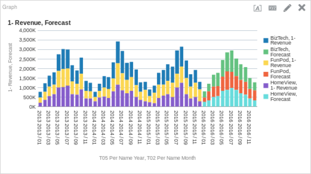
FORECAST("Base Facts"."1- Revenue", ("Time"."T05 Per Name Year", "Time"."T02 Per Name Month"), 'forecast', 'modelType=arima;numPeriods=%1;predictionInterval=%2', 12, 90)You’ll see above that I have multiple grains in my function to allow me to drill up or down, and that I am using the run-time options to determine the values of my option parameters. The “12” and “90” are the values that will seed the “%1” and “%2” options respectively. How does that look on a graph?

If you are looking to get forecasts with the least amount of input, something like the above is almost as simple as you can get. Like most other analytic functions, forecasting is an iterative process and don’t be afraid to experiment with the different options!
Always in Motion is the Future
Let’s work through a few examples to see how the function works in practice. I am using Oracle’s Sample App 607 as my sample data set for those of you following along at home (or work). Below is a more complex forecast function for the ETS model, which will forecast some operational metrics (Early Shipped Percentage in this case).
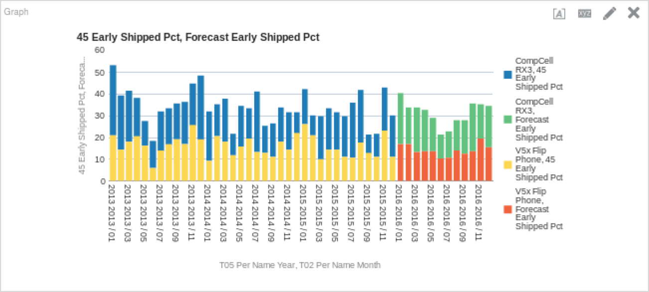
FORECAST("Simple Calculations"."45 Early Shipped Pct", ("Time"."T05 Per Name Year", "Time"."T02 Per Name Month"), 'forecast', 'numPeriods=%1;predictionInterval=90;modelType=ets;trendDamp=FALSE;errorType=A;trendType=A;seasonType=A', 12)If we are to put this on a graph, we could see something like this (depending on your filters, obviously):

Interesting, right? We can tell that the model is incorporating some of the things that we would expect from the ETS model. Because the ETS model weights data points exponentially over time, we can see that due to the relatively high performance in 2015, it will bring up our performance in 2016. We can also see that some of the seasonality is preserved as well; there are dips in performance in the summer months. Let’s do the same thing, but with the ARIMA model to see how it fares.
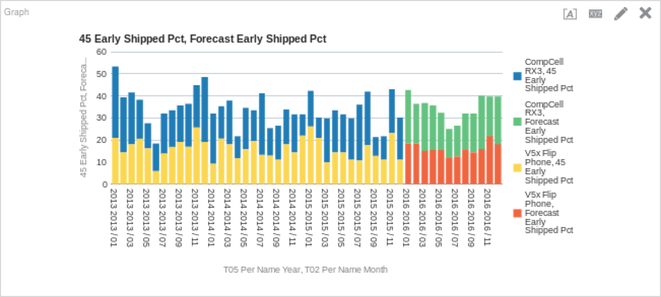
FORECAST("Simple Calculations"."45 Early Shipped Pct", ("Time"."T05 Per Name Year", "Time"."T02 Per Name Month"), 'forecast', 'numPeriods=%1;predictionInterval=90;modelType=arima', 12)
The ARIMA model looks more optimistic than the ETS model, as we can see above. This obviously will not be the case, but do keep in mind that while it is easier to configure and get an initial output, the depth of forecasting is not as deep due to the extensive list of options allowed with the ETS model. So, let’s go back to the ETS model and see how tweaking these parameters changes things.
Let’s edit the ETS model function above to see how changing these parameters impacts the forecast. I changed the ‘errorType’ and ‘trendType’ options to ‘M’ (as opposed to the prior function’s ‘A’ values). Here is the function, followed by the resultant chart.
FORECAST("Simple Calculations"."45 Early Shipped Pct", ("Time"."T05 Per Name Year", "Time"."T02 Per Name Month"), 'forecast', 'numPeriods=%1;predictionInterval=90;modelType=ets;trendDamp=FALSE;errorType=M;trendType=M;seasonType=A', 12)
It may be hard to see from the graph, but there is indeed a (minute) difference between the previous values, and the new ones.
May the Forecast Be With You
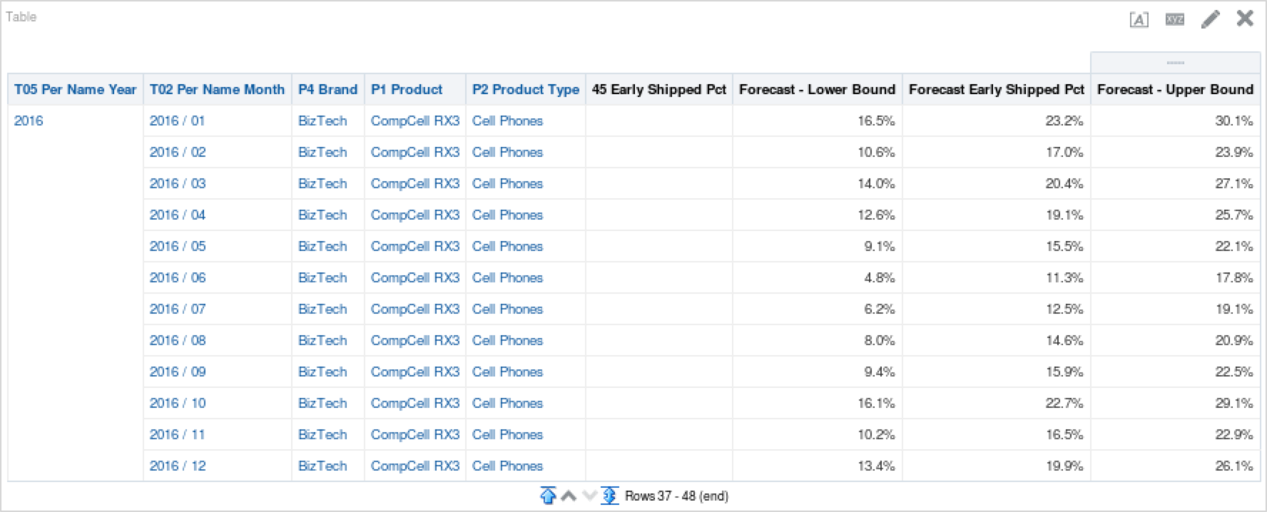
One last example I’d like to cover is using the lower and upper bounds of the forecast to add some color (and perspective) to forecasting. Lower and upper bounds are helpful because they offer a conceptual placement of where the forecast you are using is within the model’s constraints. Below are the functions I used for the lower and upper bounds for the new ETS model we just ran above. (Note: For the sake of simplicity, I am filtering the analysis further on “Product” for the “CompCell Rx3” value.)
Lower Bound:
FORECAST("Simple Calculations"."45 Early Shipped Pct", ("Time"."T05 Per Name Year", "Time"."T02 Per Name Month"), 'low', 'numPeriods=%1;predictionInterval=90;modelType=ets;trendDamp=FALSE;errorType=M;trendType=M;seasonType=A', 12)Upper Bound:
FORECAST("Simple Calculations"."45 Early Shipped Pct", ("Time"."T05 Per Name Year", "Time"."T02 Per Name Month"), 'high', 'numPeriods=%1;predictionInterval=90;modelType=ets;trendDamp=FALSE;errorType=M;trendType=M;seasonType=A', 12)And here are the results when you put it all together:

The grey line represents our modified ETS model, while the green line represents the upper bound of the model and the red is the lower bound. As I described above, this gives us a better understanding of the variance that is possible given the inputs we have provided the model to work with. We can see this forecast variability spread also if we put it into a table, as seen below.

Forecasting Has Been Known to Make Mistakes… From Time to Time
Using the new analytic functions is a different way of thinking compared to most things in OBIEE, and the Forecast function is solidly in that camp. Forecasting is an iterative process and the greater depth of detail we can give our models, the better the projections will be. While it is lunacy to assume the forecasts will be right all of the time, it can be a great tool for exposing upcoming business events, and thus allowing us to better prepare for them.